
Bring this project to life
Batch normalization is a term commonly mentioned in the context of convolutional neural networks. In this article, we are going to explore what it actually entails and its effects, if any, on the performance or overall behavior of convolutional neural networks.
import torch
import torch.nn as nn
import torch.nn.functional as F
import torchvision
import torchvision.transforms as transforms
import torchvision.datasets as Datasets
from torch.utils.data import Dataset, DataLoader
import numpy as np
import matplotlib.pyplot as plt
import cv2
from tqdm.notebook import tqdm
import seaborn as sns
from torchvision.utils import make_grid
if torch.cuda.is_available():
device = torch.device('cuda:0')
print('Running on the GPU')
else:
device = torch.device('cpu')
print('Running on the CPU')The Term Normalization
Normalization in statistics refers to the process of constraining data or a set of values between the range of 0 and 1. Rather inconveniently, in some quarters normalization also refers to the process of setting the mean of a distribution of data to zero and its standard deviation to 1.
In actual sense, this process of setting the mean of a distribution to 0 and its standard deviation to 1 is called standardization. Due to certain liberties however, it is also called normalization or z-score normalization. It is important to learn that distinction and bare it in mind.
Data Preprocessing
Data preprocessing refers to the steps taken in preparing data before being fed to a machine learning or deep learning algorithm. The two processes (normalization and standardization) mentioned in the previous section are data preprocessing steps.
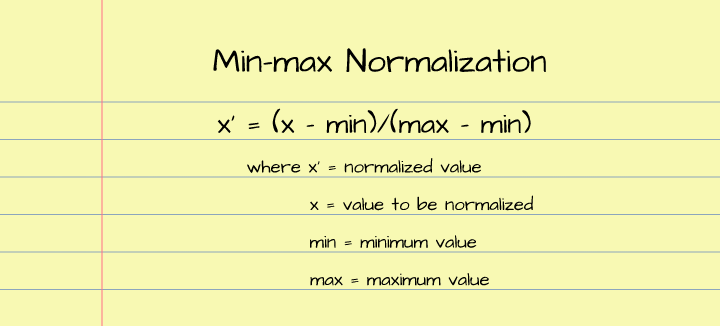
Min-max Normalization
Min-max normalization is one of the most common methods of normalizing data. Typical to its name, it constrains data points within the range of 0 and 1 by setting the minimum value in the dataset to 0, the maximum to 1 and everything in between scaled accordingly. The equation below provides a mathematical description of the min-max normalization process. Essentially it involves subtracting the minimum value in the dataset from each data point then dividing by the range (maximum - minimum).
Using the function below we can replicate the process of min-max normalization. Utilizing this function we can develop an intuition for what actually goes on behind the scenes.
def min_max_normalize(data_points: np.array):
  """
  This function normalizes data by constraining
  data points between the range of 0 & 1
  """
  #  convert list to numpy array
  if type(data_points) == list:
    data_points = np.array(data_points)
  else:
    pass

  #  create a list to hold normalized data
  normalized = []

  #  derive minimum and maximum values
  minimum = data_points.min()
  maximum = data_points.max()

  #  convert to list for iteration
  data_points = list(data_points)
  #  normalizing data
  for value in data_points:
    normalize = (value-minimum)/(maximum-minimum)
    normalized.append(round(normalize, 2))

  return np.array(normalized)
Lets create an array of random values using NumPy then attempt to normalize them using the min-max normalization function defined above.
#  creating a random set of data points
data = np.random.rand(50)*20

#  normalizing data points
normalized = min_max_normalize(data)
From the plots below, it can be seen that before normalization, values ranged from o to 20 with a vast majority of data points having values between 5 and 10. After normalization however, it can be seen that values now range between 0 and 1 with a vast majority of data points having values between 0.25 and 0.5. Note: if/when you run this code the data distribution will be different from what is used in this article as it is randomly generated.
#  visualising distribution
figure, axes = plt.subplots(1, 2, sharey=True, dpi=100)
sns.histplot(data, ax=axes[0])
axes[0].set_title('unnormalized')
sns.histplot(normalized, ax=axes[1])
axes[1].set_title('min-max normalized')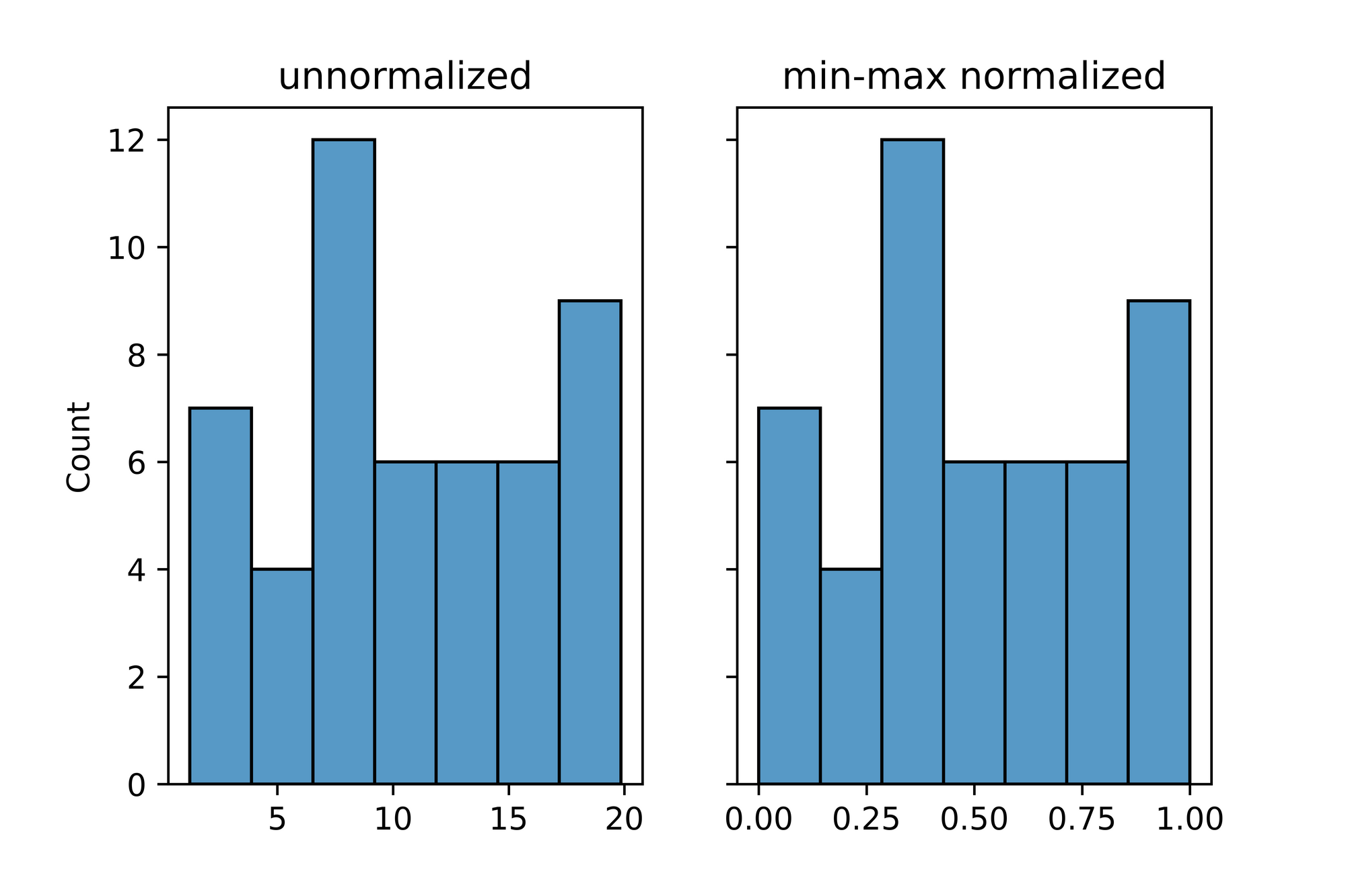
Z-score Normalization
Z-score normalization, also called standardization, is the process of setting the mean and standard deviation of a data distribution to 0 and 1 respectively. The equation below is the mathematical equation which governs z-score normalization, it involves subtracting the mean of the distribution from the value to be normalized before dividing by the distribution's standard deviation.

The function defined below replicates the z-score normalization process, with this function we can take a closer look at what it actually entails.
def z_score_normalize(data_points: np.array):
  """
  This function normalizes data by computing
  their z-scores
  """
  #  convert list to numpy array
  if type(data_points) == list:
    data_points = np.array(data_points)
  else:
    pass

  #  create a list to hold normalized data
  normalized = []

  #  derive mean and and standard deviation
  mean = data_points.mean()
  std = data_points.std()

  #  convert to list for iteration
  data_points = list(data_points)
  #  normalizing data
  for value in data_points:
    normalize = (value-mean)/std
    normalized.append(round(normalize, 2))

  return np.array(normalized)
Using the data distribution generated in the previous section, let us attempt to normalize the data points using the z-score function.
#  normalizing data points
z_normalized = z_score_normalize(data)

#  check the mean value
z_normalized.mean()
>>>> -0.0006

#  check the standard deviation
z_normalized.std()
>>>> 1.0000
Again, from the visualizations, we can see that the the original distribution has values ranging from 0 to 20 while the z-score normalized values are now centered around 0 (a mean of zero) and a range of approximately -1.5 to 1.5 which is a more manageable range.
#  visualizing distributions
figure, axes = plt.subplots(1, 2, sharey=True, dpi=100)
sns.histplot(data, ax=axes[0])
axes[0].set_title('unnormalized')
sns.histplot(z_normalized, ax=axes[1])
axes[1].set_title('z-score normalized')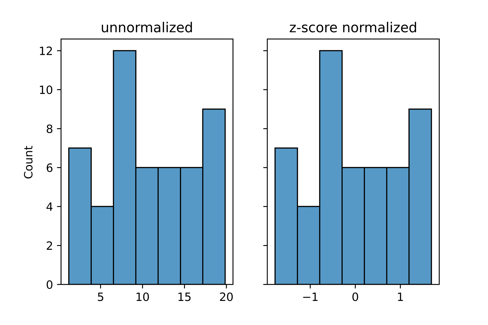
Reasons for Preprocessing
When regarding data in machine learning, we look at individual data points as features. All of these features are typically not on the same scale scale. For instance, consider a house with 3 bedrooms and a sitting room of size 400 square feet. These two features are on scales so far apart that if they are feed into a machine learning algorithm slated to be optimized by gradient descent. Optimization would be quite tedious, as the feature with the bigger scale will take precedent over all others. In order to ease the optimization process, it is a good idea to have all data points within the same scale.
Normalization in Convolution Layers
The data points in an image are its pixels. Pixel values typically range from 0 to 255; which is why, before feeding images into a convolutional neural network, it is a good idea to normalize them in some way so as to put all pixels in a manageable range.
Even when this is done, when training a convnet, weights (elements in its filters) might become too large, and thereby produce feature maps with pixels spread across a wide range. This essentially renders the normalization done during the preprocessing step somewhat futile. Furthermore, this could hamper the optimization process making it slow or in extreme cases it could lead to a problem called unstable gradients, which could essentially prevent the convnet from further optimizing it's weights entirely.
In order to prevent this problem, a normalization is introduced in each layer of the convent. This normalization is termed Batch Normalization.
The Process of Batch Normalization
Batch normalization essentially sets the pixels in all feature maps in a convolution layer to a new mean and a new standard deviation. Typically, it starts off by z-score normalizing all pixels, and then goes on to multiply the normalized values by an arbitrary parameter alpha (scale) before adding another arbitrary parameter beta (offset).
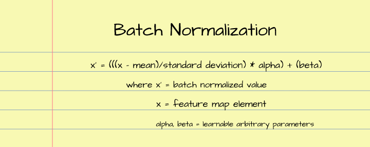
These two parameters alpha and beta are learnable parameters which the convnet will then use to ensure that pixel values in the feature maps are within a manageable range - thereby ameliorating the problem of unstable gradients.
Batch Normalization in Action
In order to really assess the effects of batch normalization in convolution layers, we need to benchmark two convnets, one without batch normalization and the other with batch normalization. For this we will be using the LeNet-5 architecture and the MNIST dataset.
Bring this project to life
Dataset & Convolutional Neural Network Class
In this article, the MNIST dataset will be used for benchmarking purposes as mentioned previously. This dataset consists of 28 x 28 pixel images of handwritten digits ranging from digit 0 to 9 labelled accordingly.
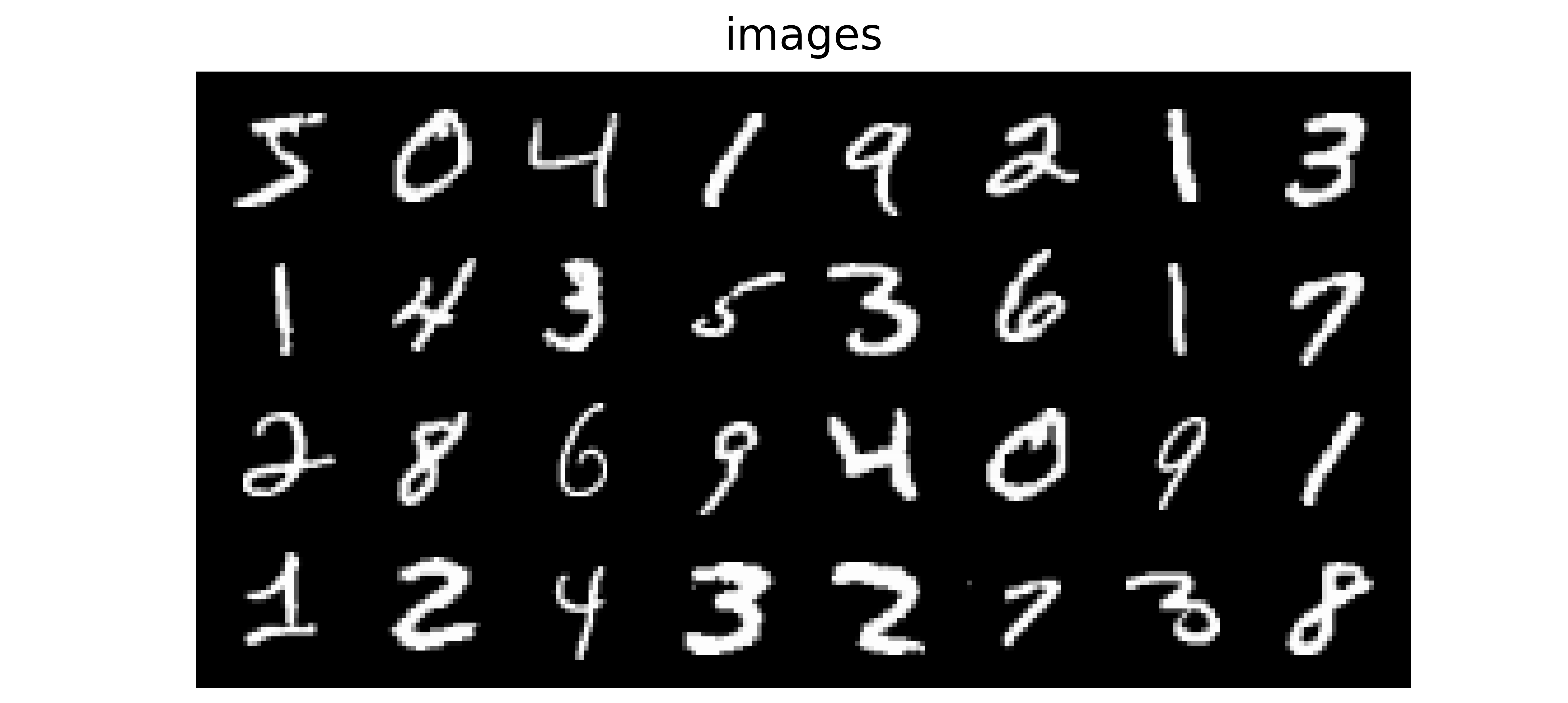
It can be loaded in PyTorch using the code block below. The training set is comprised of 60,000 images while the validation set is made up of 10,000 images. Since we will be using this dataset with LeNet-5, the images need to be resized to 32 x 32 pixels as defined in the transforms parameter.
#  loading training data
training_set = Datasets.MNIST(root='./', download=True,
                              transform=transforms.Compose([transforms.ToTensor(),
                                                            transforms.Resize((32, 32))]))

#  loading validation data
validation_set = Datasets.MNIST(root='./', download=True, train=False,
                                transform=transforms.Compose([transforms.ToTensor(),
                                                              transforms.Resize((32, 32))]))
For training and utilization of our convnets, we shall be using the class below aptly named 'ConvolutionalNeuralNet()'. This class contains methods which will help to train and classify instances using the trained convnet. The train() method also contains inner helper functions such as init_weights() and accuracy.
class ConvolutionalNeuralNet():
  def __init__(self, network):
    self.network = network.to(device)
    self.optimizer = torch.optim.Adam(self.network.parameters(), lr=1e-3)

  def train(self, loss_function, epochs, batch_size,
            training_set, validation_set):

    #  creating log
    log_dict = {
        'training_loss_per_batch': [],
        'validation_loss_per_batch': [],
        'training_accuracy_per_epoch': [],
        'validation_accuracy_per_epoch': []
    }

    #  defining weight initialization function
    def init_weights(module):
      if isinstance(module, nn.Conv2d):
        torch.nn.init.xavier_uniform_(module.weight)
        module.bias.data.fill_(0.01)
      elif isinstance(module, nn.Linear):
        torch.nn.init.xavier_uniform_(module.weight)
        module.bias.data.fill_(0.01)

    #  defining accuracy function
    def accuracy(network, dataloader):
      network.eval()
      total_correct = 0
      total_instances = 0
      for images, labels in tqdm(dataloader):
        images, labels = images.to(device), labels.to(device)
        predictions = torch.argmax(network(images), dim=1)
        correct_predictions = sum(predictions==labels).item()
        total_correct+=correct_predictions
        total_instances+=len(images)
      return round(total_correct/total_instances, 3)

    #  initializing network weights
    self.network.apply(init_weights)

    #  creating dataloaders
    train_loader = DataLoader(training_set, batch_size)
    val_loader = DataLoader(validation_set, batch_size)

    #  setting convnet to training mode
    self.network.train()

    for epoch in range(epochs):
      print(f'Epoch {epoch+1}/{epochs}')
      train_losses = []

      #  training
      print('training...')
      for images, labels in tqdm(train_loader):
        #  sending data to device
        images, labels = images.to(device), labels.to(device)
        #  resetting gradients
        self.optimizer.zero_grad()
        #  making predictions
        predictions = self.network(images)
        #  computing loss
        loss = loss_function(predictions, labels)
        log_dict['training_loss_per_batch'].append(loss.item())
        train_losses.append(loss.item())
        #  computing gradients
        loss.backward()
        #  updating weights
        self.optimizer.step()
      with torch.no_grad():
        print('deriving training accuracy...')
        #  computing training accuracy
        train_accuracy = accuracy(self.network, train_loader)
        log_dict['training_accuracy_per_epoch'].append(train_accuracy)

      #  validation
      print('validating...')
      val_losses = []

      #  setting convnet to evaluation mode
      self.network.eval()

      with torch.no_grad():
        for images, labels in tqdm(val_loader):
          #  sending data to device
          images, labels = images.to(device), labels.to(device)
          #  making predictions
          predictions = self.network(images)
          #  computing loss
          val_loss = loss_function(predictions, labels)
          log_dict['validation_loss_per_batch'].append(val_loss.item())
          val_losses.append(val_loss.item())
        #  computing accuracy
        print('deriving validation accuracy...')
        val_accuracy = accuracy(self.network, val_loader)
        log_dict['validation_accuracy_per_epoch'].append(val_accuracy)

      train_losses = np.array(train_losses).mean()
      val_losses = np.array(val_losses).mean()

      print(f'training_loss: {round(train_losses, 4)}  training_accuracy: '+
      f'{train_accuracy}  validation_loss: {round(val_losses, 4)} '+
      f'validation_accuracy: {val_accuracy}\n')

    return log_dict

  def predict(self, x):
    return self.network(x)
Lenet-5
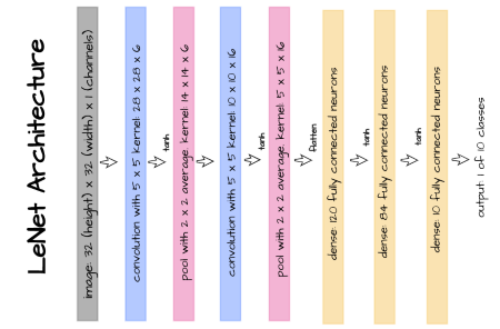
LeNet-5 (Y. Lecun et al) is one of the earliest convolutional neural networks specifically designed to recognize/classify images of hand written digits. Its architecture is depicted in the image above and its implementation in PyTorch is provided in the following code block.
class LeNet5(nn.Module):
  def __init__(self):
    super().__init__()
    self.conv1 = nn.Conv2d(1, 6, 5)
    self.pool1 = nn.AvgPool2d(2)
    self.conv2 = nn.Conv2d(6, 16, 5)
    self.pool2 = nn.AvgPool2d(2)
    self.linear1 = nn.Linear(5*5*16, 120)
    self.linear2 = nn.Linear(120, 84)
    self.linear3 = nn. Linear(84, 10)

  def forward(self, x):
    x = x.view(-1, 1, 32, 32)

    #----------
    # LAYER 1
    #----------
    output_1 = self.conv1(x)
    output_1 = torch.tanh(output_1)
    output_1 = self.pool1(output_1)

    #----------
    # LAYER 2
    #----------
    output_2 = self.conv2(output_1)
    output_2 = torch.tanh(output_2)
    output_2 = self.pool2(output_2)

    #----------
    # FLATTEN
    #----------
    output_2 = output_2.view(-1, 5*5*16)

    #----------
    # LAYER 3
    #----------
    output_3 = self.linear1(output_2)
    output_3 = torch.tanh(output_3)

    #----------
    # LAYER 4
    #----------
    output_4 = self.linear2(output_3)
    output_4 = torch.tanh(output_4)

    #-------------
    # OUTPUT LAYER
    #-------------
    output_5 = self.linear3(output_4)
    return(F.softmax(output_5, dim=1))
Using the above defined LeNet-5 architecture, we will instantiate model_1, a member of the ConvolutionalNeuralNet class, with parameters as seen in the code block. This model will serve as our baseline for benchmarking purposes.
#  training model 1
model_1 = ConvolutionalNeuralNet(LeNet5())

log_dict_1 = model_1.train(nn.CrossEntropyLoss(), epochs=10, batch_size=64,
                       training_set=training_set, validation_set=validation_set)
After training for 10 epochs and visualizing accuracies from the metric log we receive in return, we can see that both training and validation accuracy increased over the course of training. In our experiment, validation accuracy started off at approximately 93% after the first epoch before proceeding to increase steadily over the next 9 iterations, eventually terminating at just over 98% by epoch 10.
sns.lineplot(y=log_dict_1['training_accuracy_per_epoch'], x=range(len(log_dict_1['training_accuracy_per_epoch'])), label='training')

sns.lineplot(y=log_dict_1['validation_accuracy_per_epoch'], x=range(len(log_dict_1['validation_accuracy_per_epoch'])), label='validation')

plt.xlabel('epoch')
plt.ylabel('accuracy')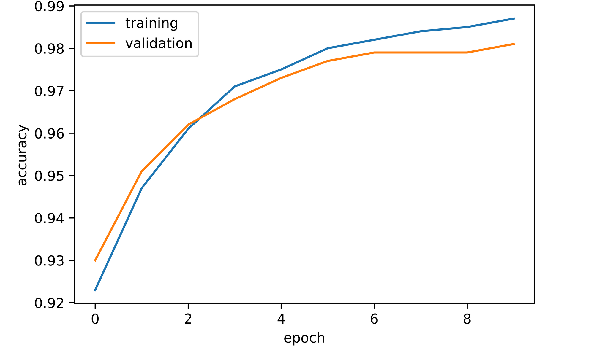
Batch Normalized LeNet-5
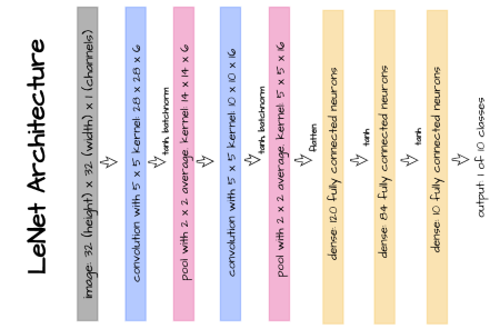
Since the theme of this article is centered around batch normalization in convolution layers, batch norm is only applied on the two convolution layers present in this architecture as illustrated in the image above.
class LeNet5_BatchNorm(nn.Module):
  def __init__(self):
    super().__init__()
    self.conv1 = nn.Conv2d(1, 6, 5)
    self.batchnorm1 = nn.BatchNorm2d(6)
    self.pool1 = nn.AvgPool2d(2)
    self.conv2 = nn.Conv2d(6, 16, 5)
    self.batchnorm2 = nn.BatchNorm2d(16)
    self.pool2 = nn.AvgPool2d(2)
    self.linear1 = nn.Linear(5*5*16, 120)
    self.linear2 = nn.Linear(120, 84)
    self.linear3 = nn. Linear(84, 10)

  def forward(self, x):
    x = x.view(-1, 1, 32, 32)

    #----------
    # LAYER 1
    #----------
    output_1 = self.conv1(x)
    output_1 = torch.tanh(output_1)
    output_1 = self.batchnorm1(output_1)
    output_1 = self.pool1(output_1)

    #----------
    # LAYER 2
    #----------
    output_2 = self.conv2(output_1)
    output_2 = torch.tanh(output_2)
    output_2 = self.batchnorm2(output_2)
    output_2 = self.pool2(output_2)

    #----------
    # FLATTEN
    #----------
    output_2 = output_2.view(-1, 5*5*16)

    #----------
    # LAYER 3
    #----------
    output_3 = self.linear1(output_2)
    output_3 = torch.tanh(output_3)

    #----------
    # LAYER 4
    #----------
    output_4 = self.linear2(output_3)
    output_4 = torch.tanh(output_4)

    #-------------
    # OUTPUT LAYER
    #-------------
    output_5 = self.linear3(output_4)
    return(F.softmax(output_5, dim=1))
Using the code segment below, we can nstantiate model_2 with batch normalization included, and begin training with the same parameters as model_1. Then, we yield accuracy scores..
# training model 2
model_2 = ConvolutionalNeuralNet(LeNet5_BatchNorm())
log_dict_2 = model_2.train(nn.CrossEntropyLoss(), epochs=10, batch_size=64,
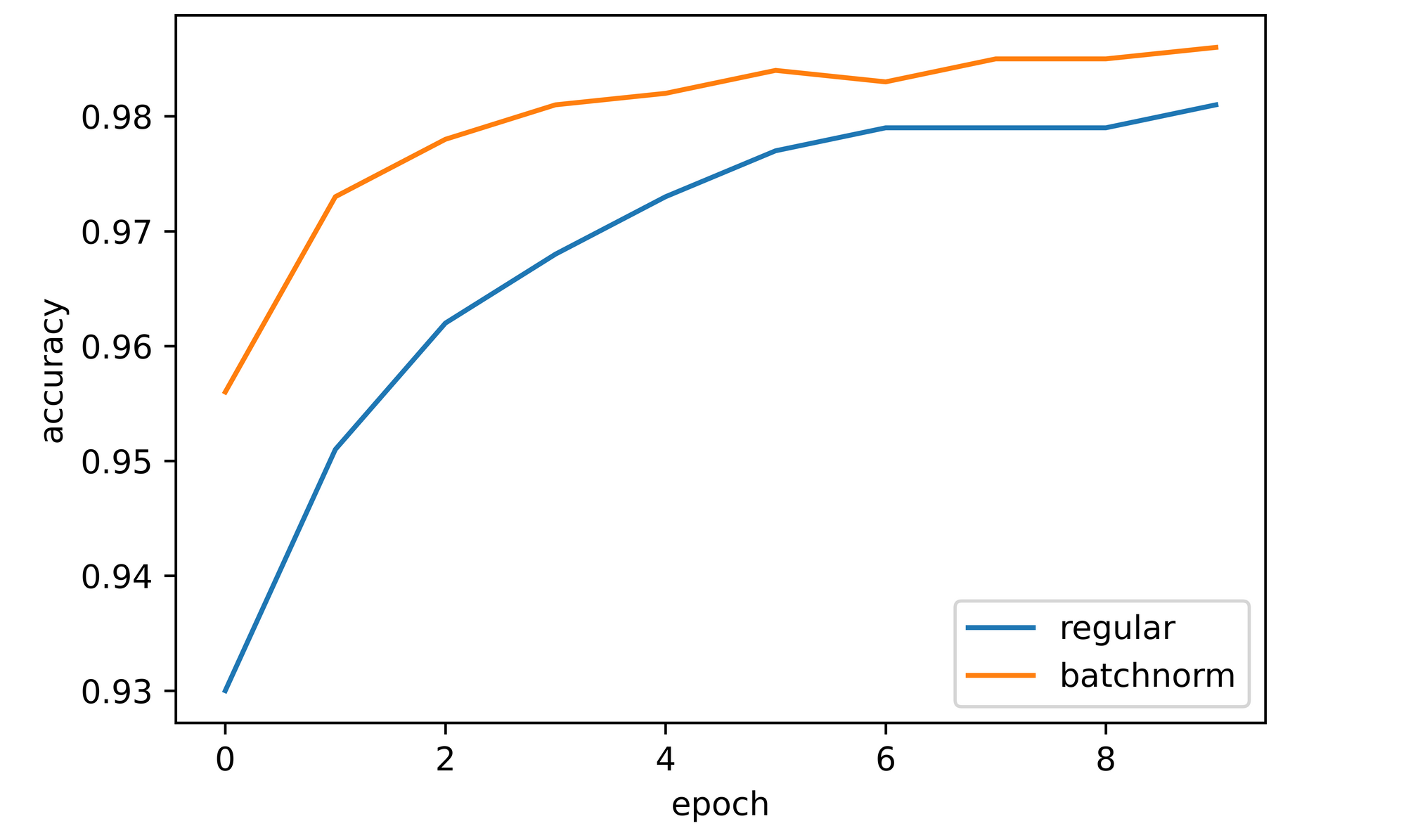
training_set=training_set, validation_set=validation_set)Looking at the plot, it is clear that both training and validation accuracies increased over the course of training similar to the model without batch normalization. Validation accuracy after the first epoch stood at just above 95%, 3 percentage points higher than model_1 at the same point, before increasing gradually and culminating at approximately 98.5%, 0.5% higher than model_1.
sns.lineplot(y=log_dict_2['training_accuracy_per_epoch'], x=range(len(log_dict_2['training_accuracy_per_epoch'])), label='training')

sns.lineplot(y=log_dict_2['validation_accuracy_per_epoch'], x=range(len(log_dict_2['validation_accuracy_per_epoch'])), label='validation')

plt.xlabel('epoch')
plt.ylabel('accuracy')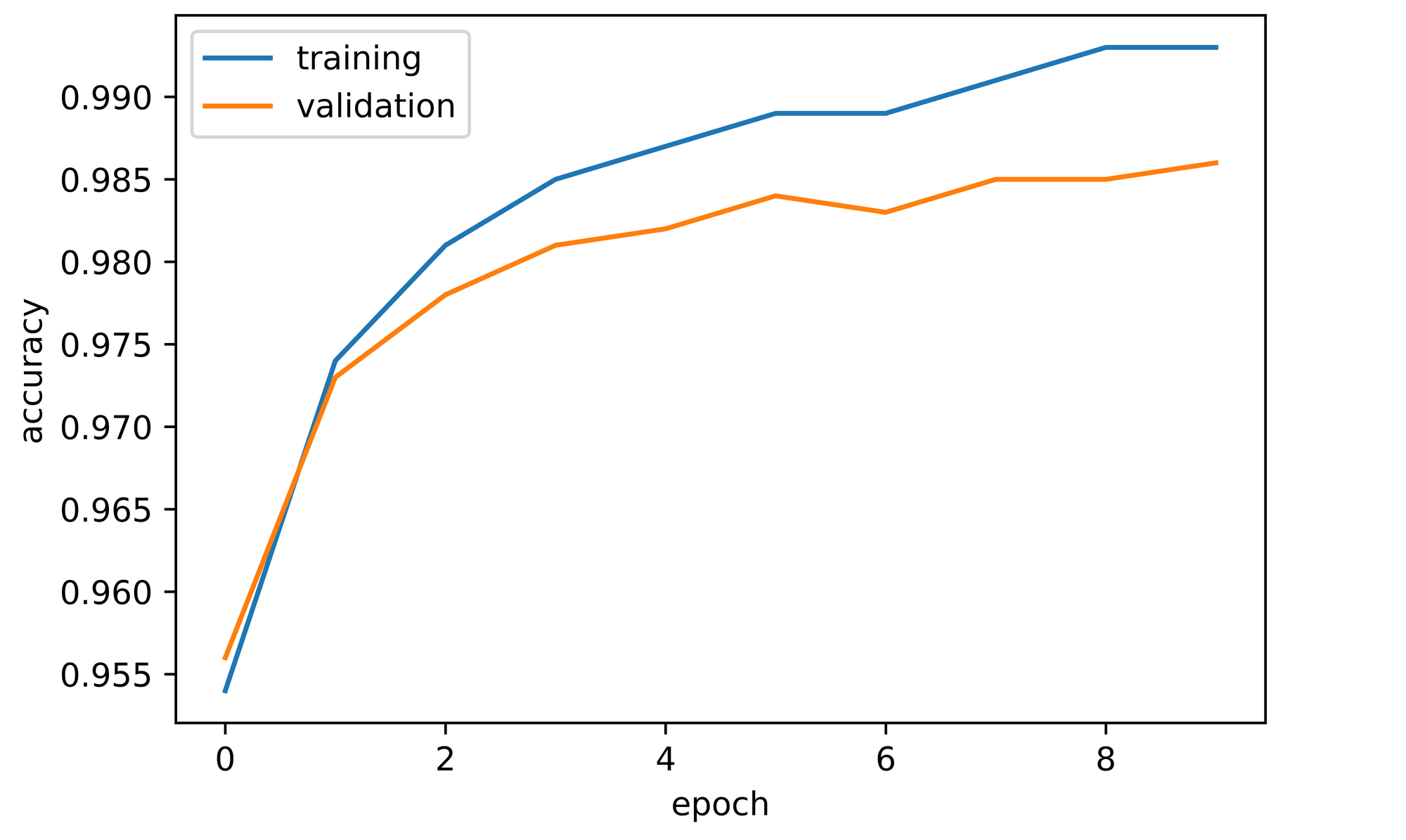
Comparing Models
Comparing both models, it is clear that the LeNet-5 model with batch normalized convolution layers outperformed the regular model without batch normalized convolution layers. It is therefore safe to say that batch normalization has lent a hand to increasing performance in this instance.
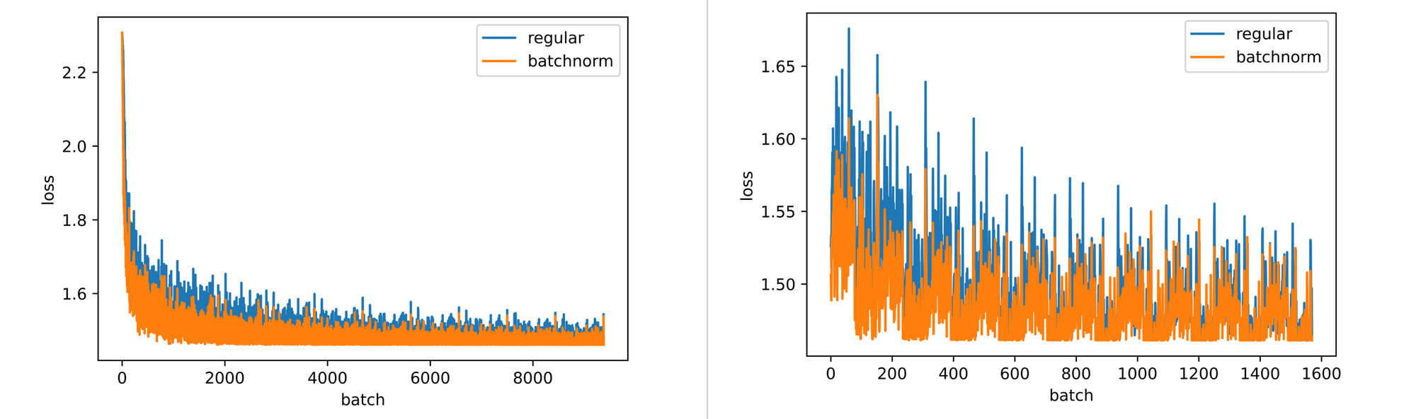
Comparing training and validation losses between the regular and batch normalized LeNet-5 models also shows that the batch normalized model attains lower loss values faster than the regular model. This is a pointer to batch normalization increasing the rate at which the model optimizes it's weights in the correct direction or in other words, batch normalization increases the rate at which the convnet learns.
Final Remarks
In this article, we explored what normalization entails in a machine learning/deep learning context. We also explored normalization processes as data preprocessing steps and how normalization can be taken beyond preprocessing and into convolution layers via the process of batch normalization.
Afterwards, we examined the process of batch normalization itself before assessing it's effects by benchmarking two variations of LeNet-5 convnets (one without batch norm and the other with batch norm) on the MNIST dataset. From the results, we inferred that batch normalization contributed to an increase in performance and weight optimization speed. There have also been some suggestions that it prevents internal covariate shift however a concensus might as well not have been reached on that.