
In a previous article we discussed the theory behind Bayesian Decision Theory in detail. In this article we'll see how to apply Bayesian Decision Theory to different classification problems. We'll discuss concepts like the loss and risk of doing a classification problem, and how they're done in a step-by-step manner. To handle the uncertainty in making a classification, the "reject class" is also discussed. Any sample with a weak posterior probability is assigned to the reject class. We'll conclude by analyzing the conditions under which a sample is classified as a reject.
The outline of this article is as follows:
- Quick Review of Bayesian Decision Theory
- Bayesian Decision Theory with Binary Classes
- Bayesian Decision Theory with Multiple Classes
- Loss & Risk
- 0/1 Loss
- Example to Calculate Risk
- Reject Class
- When to Classify Samples As Rejects?
- Conclusion
Let's get started.
Bring this project to life
Quick Review of Bayesian Decision Theory
In a previous article we discussed Bayesian Decision Theory in detail, including the prior, likelihood, and posterior probabilities. The posterior probability is calculated according to this equation:
$$ P(C_i|X)=\frac{P(C_i)P(X|C_i)}{P(X)} $$
The evidence $P(X)$ in the denominator can be calculated as follows:
$$ P(X)=\sum_{i=1}^{K}P(X|C_i)P(C_i) $$
As a result, the first equation can be written as follows:
$$ P(C_i|X)=\frac{P(C_i)P(X|C_i)}{\sum_{k=1}^{K}P(X|C_k)P(C_k)} $$
We also showed that the sum of prior probabilities must be 1:
$$ \sum_{i=1}^{K}P(C_i)=1 $$
The same is true for the posterior probabilities:
$$ \sum_{i=1}^{K}P(C_i|X)=1 $$
We ended the first article by mapping the concepts from Bayesian Decision Theory to the context of machine learning. According to this discussion, it was shown that the prior, likelihood, and evidence play an important role in making a good prediction that takes into consideration the following aspects:
- The prior probability $P(C_i)$ reflects how the model is trained by samples from class $C_i$.
- The likelihood probability $P(X|C_i)$ refers to the model's knowledge in classifying the sample $X$ as the class $C_i$.
- The evidence term $P(X)$ shows how much the model knows about the sample $X$.
Now let's discuss how to do classification problems using Bayesian Decision Theory.
Bayesian Decision Theory with Binary Classes
For a binary classification problem, the posterior probability of the two classes are calculated as follows:
$$ P(C_1|X)=\frac{P(C_1)P(X|C_1)}{\sum_{k=1}^{K}P(X|C_k)P(C_k)}
\\
P(C_2|X)=\frac{P(C_2)P(X|C_2)}{\sum_{k=1}^{K}P(X|C_k)P(C_k)} $$
The sample is classified according to the class with the highest posterior probability.
For binary classification problems, the posterior probability for only one class can be enough. This is because the sum of all posterior probabilities is 1:
$$ P(C_1|X)+P(C_2|X)=1
\\
P(C_1|X)=1-P(C_2|X)
\\
P(C_2|X)=1-P(C_1|X) $$
Given the posterior probability of one class, the posterior probability of the second class is thus also known. For example, if the posterior probability for class $C_1$ is 0.4, then the posterior probability for the other class $C_2$ is:
$$ 1.0-0.4=0.6 $$
It is also possible to calculate the posterior probabilities of all classes, and compare them to determine the output class.
$$ C_1 \space if \space P(C_1|X)>P(C_2|X)
\\
C_2 \space if \space P(C_2|X)>P(C_1|X) $$
Bayesian Decision Theory with Multiple Classes
For a multi-class classification problem, the posterior probability is calculated for each of the classes. The sample is classified according to the class with the highest probability.
Assuming there are 3 classes, here is the posterior probability for each:
$$ P(C_1|X)=\frac{P(C_1)P(X|C_1)}{\sum_{k=1}^{K}P(X|C_k)P(C_k)}
\\
P(C_2|X)=\frac{P(C_2)P(X|C_2)}{\sum_{k=1}^{K}P(X|C_k)P(C_k)}
\\
P(C_3|X)=\frac{P(C_3)P(X|C_3)}{\sum_{k=1}^{K}P(X|C_k)P(C_k)} $$
Based on the posterior probabilities of these 3 classes, the input sample $X$ is assigned to the class with the highest posterior probability.
$$ max \space [P(C_1|X), P(C_2|X), P(C_3|X)] $$
If the probabilities of the 3 classes are 0.2, 0.3, and 0.5, respectively, then the input sample is assigned to the third class $C_3$.
$$ Choose \space C_i \space\ if \space P(C_i|X) = max_k \space P(C_k|X), \space k=1:K $$
Loss and Risk
For a given sample that belongs to the class $C_k$, Bayesian Decision Theory may take an action that classifies the sample as belonging to class $\alpha_i$ which has the highest posterior probability.
The action (i.e. classification) is correct when $i=k$. In other words:
$$ C_k=\alpha_i $$
It may happen that the predicted class $\alpha_i$ is different from the correct class $C_k$. As a result of this wrong action (i.e. classification), there is a loss. The loss is denoted as lambda $\lambda$:
$$ loss = \lambda_{ik} $$
Where $i$ is the index of the predicted class and $k$ is the index of the correct class.
Due to the possibility of taking an incorrect action (i.e. classification), there is a risk (i.e. cost) for taking the wrong action. Risk $R$ is calculated as follows:
$$ R(\alpha_{i}|X)=\sum_{k=1}^{K}\lambda_{ik}P(C_k|X) $$
The goal is to choose the class that reduces the risk. This is formulated as follows:
$$ Choose \space \alpha_i \space\ so \space that \space R(\alpha_i|X) = min_k \space R(\alpha_k|X), \space k=1:K $$
Note that the loss is a metric that shows whether a single prediction is correct or incorrect. Based on the loss, the risk (i.e. cost) is calculated, which is a metric that shows how the overall model predictions are correct or incorrect. The lower the risk, the better the model is at making predictions.
0/1 Loss
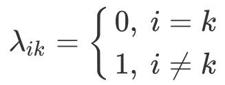
There are different ways to calculate the loss. One way is by using the "0/1 loss". When the prediction is correct, then the loss is $0$ (i.e. there is no loss). When there is a wrong prediction, then the loss is always $1$.
The 0/1 loss is modeled below, where $i$ is the index of the wrong class and $k$ is the index of the correct class.
Remember that the risk is calculated as follows:
$$ R(\alpha_{i}|X)=\sum_{k=1}^{K}\lambda_{ik}P(C_k|X) $$
Based on the 0/1 loss, the loss is only $0$ or $1$. As a result, the loss term $\lambda$ can be removed from the risk equation. The risk is calculated as follows, by excluding the posterior probability from the summation when $k=i$:
$$ R(\alpha_i|X) = \sum_{k=1, k\not=i}^{K} P(C_k|X) $$
Whenever i not equal k, then there is a wrong classification (action) and the loss is 1. Thus, the risk is incremented by the posterior probability of the wrong class.
If we don't remove $\lambda$, then it multiplies the posterior probability of the current class $i$ by 0. Thus we exclude it from the summation. After removing $\lambda$, it is important to manually exclude the posterior probability of the current class $i$ from the summation. This is why the summation does not include the posterior probability when $k=i$.
The previous equation calculates the sum of all posterior probabilities except for the posterior probability of class $i$. Because the sum of all posterior probabilities is 1, the following equation holds:
$$ [\sum_{k=1, k\not=i}^{K} P(C_k|X)]+P(C_i|X)=1 $$
By keeping the sum of posterior probabilities of all classes (except for the class $i$) on one side, here is the result:
$$ \sum_{k=1, k\not=i}^{K} P(C_k|X)=1-P(C_i|X) $$
As a result, the risk of classifying the sample as class $i$ becomes:
$$ R(\alpha_i|X) = 1-P(C_i|X) $$
According to this equation, the risk is minimized when the class with the highest posterior probability is selected. Thus, we should work on maximizing the posterior probability.
As a summary, here are the different ways to calculate the risk of taking an action given that the 0/1 loss is used:
$$ R(\alpha_i|X) = \sum_{k=1}^{K}\lambda_{ik} P(C_k|X)
\\R(\alpha_i|X) = \sum_{k=1,k\not=i}^{K} P(C_k|X)
\\R(\alpha_i|X) = 1-P(C_i|X) $$
Here are some notes about the 0/1 loss:
- Based on the 0/1 loss, all the incorrect actions (i.e. classifications) are given equal losses of $1$, and all correct classifications have no losses (e.g. $0$ loss). For example, if there are 4 wrong classifications, then the total loss is $4(1)=4$.
- It is not perfect to assign equal losses to all incorrect predictions. The loss should increases proportionally to the posterior probability of the wrong class. For example, the loss in the case of a wrong prediction with a posterior probability of 0.8 should be higher than when the posterior probability is just 0.2.
- The 0/1 loss assigns 0 loss to the correct predictions. However, it may happen to add a loss to the correct predictions when the posterior probability is low. For example, assume the correct class is predicted with a posterior probability of 0.3, which is small. The loss function may add a loss to penalize the predictions with low confidence, even though they are correct.
Example to Calculate Risk
Assume there are just two classes, $C_1$ and $C_2$, where their posterior probabilities are:
$$ P(C_1|X)=0.1
\\
P(C_2|X)=0.9 $$
How do we select the predicted class? Remember that the objective is to select the class that minimizes the risk. It is formulated as follows:
$$ Choose \space \alpha_i \space\ so \space that \space R(\alpha_i|X) = min_k \space R(\alpha_k|X), \space k=1:K $$
So, to decide which class to select, we can easily calculate the risk in case of predicting $C_1$ and $C_2$. Remember that the risk is calculated as follows:
$$ R(\alpha_i|X) = 1-P(C_i|X) $$
For $C_1$, its posterior probability is 0.1, and thus the risk of classifying the sample $X$ as the class $C_1$ is 0.9.
$$ R(\alpha_1|X) = 1-P(C_1|X) = 1-0.1=0.9 $$
For $C_2$, its posterior probability is 0.9, and thus the risk of classifying the sample $X$ as the class $C_2$ is 0.1.
$$ R(\alpha_2|X) = 1-P(C_2|X) = 1-0.9=0.1 $$
The risks of classifying the input sample as $C_1$ and $C_2$ are 0.9 and 0.1, respectively. Because the objective is to select the class that minimizes the risk, the selected class is thus $C_2$. In other words, the input sample $X$ is classified as the class $C_2$.
Reject Class
Previously, when there was a wrong action (i.e. classification), its posterior probability was incorporated into the risk. But still, the wrong action was taken. Sometimes, we do not need to take the wrong action at all.
For example, imagine an employee who sends letters according to postal codes. Sometimes the employee may take wrong actions by sending envelopes to the incorrect homes. We need to avoid this action. This can be accomplished by adding a new reject class to the set of available classes.
Rather than having only $K$ classes, there are now $K+1$ classes. The $K+1$ class is the reject class, and the classes from $k=1$ to $k=K$ are the normal classes. The reject class has a loss equal to $\lambda$, which is between 0 and 1 (exclusive).
The reject action is given the index $k+1$ as follows:
$$ C_{reject}=\alpha_{K+1} $$
When the reject class exists, here is the 0/1 loss function for choosing class $i$ when the correct class is $k$:
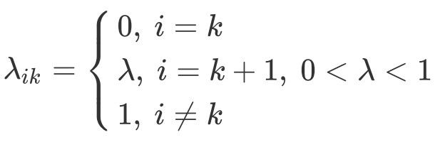
The risk of classifying $X$ as the reject class is:
$$ R(\alpha_{K+1}|X) = \sum_{k=1}^{K}\lambda P(C_k|X) $$
The summation operator can be factored as follows:
$$ R(\alpha_{k+1}|X) = \lambda P(C_1|X) + \lambda P(C_2|X) +...+ \lambda P(C_K|X) $$
By taking out $\lambda$ as a common factor, the result is:
$$ R(\alpha_{K+1}|X) = \lambda [P(C_1|X) + P(C_2|X) +...+ P(C_K|X)] $$
Because the sum of all (from 1 to K) posterior probabilities is 1, then the following holds:
$$ P(C_1|X) + P(C_2|X) +...+ P(C_K|X)=1 $$
As a result, the risk of classifying $X$ according to the reject class is $\lambda$:
$$ R(\alpha_{K+1}|X) = \lambda $$
Remember that the risk of choosing a class $i$ other than the reject class is:
$$ R(\alpha_{i}|X) = \sum_{k=1}^{K}\lambda_{ik} P(C_k|X)= \sum_{k=1, \forall k\not = i}^{K} P(C_k|X) = 1-P(C_i|X) $$
When to Classify Samples As Rejects?
This is an important question. When should we classify a sample as class $i$, or the reject class?
Class $C_i$ is selected when the following 2 conditions hold:
- The posterior probability of classifying the sample as class $C_i$ is higher than the posterior probabilities of all other classes.
- The posterior probability of class $C_i$ is higher than the threshold $1-\lambda$.
These 2 conditions are modeled as follows:
$$ Choose \space C_i \space\ if \space [P(C_i|X)>P(C_{k, k\not=i}|X)] \space AND \space [P(C_i|X)>P(C_{reject}|X)]
\\
Otherwise, \space choose \space Reject \space\ class $$
The condition $0 < \lambda < 1$ must be satisfied for the following 2 reasons:
- If $\lambda=0$, then the threshold is $1-\lambda = 1-0 = 1$, which means a sample is classified as class $C_i$ only when the posterior probability is higher than 1. As a result, all samples are classified as the reject class because the posterior probability cannot be higher than 1.
- If $\lambda=1$, then the threshold is $1-\lambda = 1-1 = 0$, which means a sample is classified as class $C_i$ only when the posterior probability is higher than 0. As a result, the majority of samples will be classified as belonging to the class $C_i$ because the majority of the posterior probabilities are higher than 0. Only samples with a posterior probability of 0 are assigned to the reject class.
Conclusion
In these two articles, Bayesian Decision Theory was introduced in a detailed step-by-step manner. The first article covered how the prior and likelihood probabilities are used to form the theory. In this article we saw how to apply Bayesian Decision Theory to binary and multi-class classification problems. We described how the binary and multi-class losses are calculated, how the predicted class is derived based on the posterior probabilities, and how the risk/cost is calculated. Finally, the reject class was introduced to handle uncertainty.