Kolmogorov-Arnold Networks (KAN): Promising Alternative to Multi-Layer Perceptron?

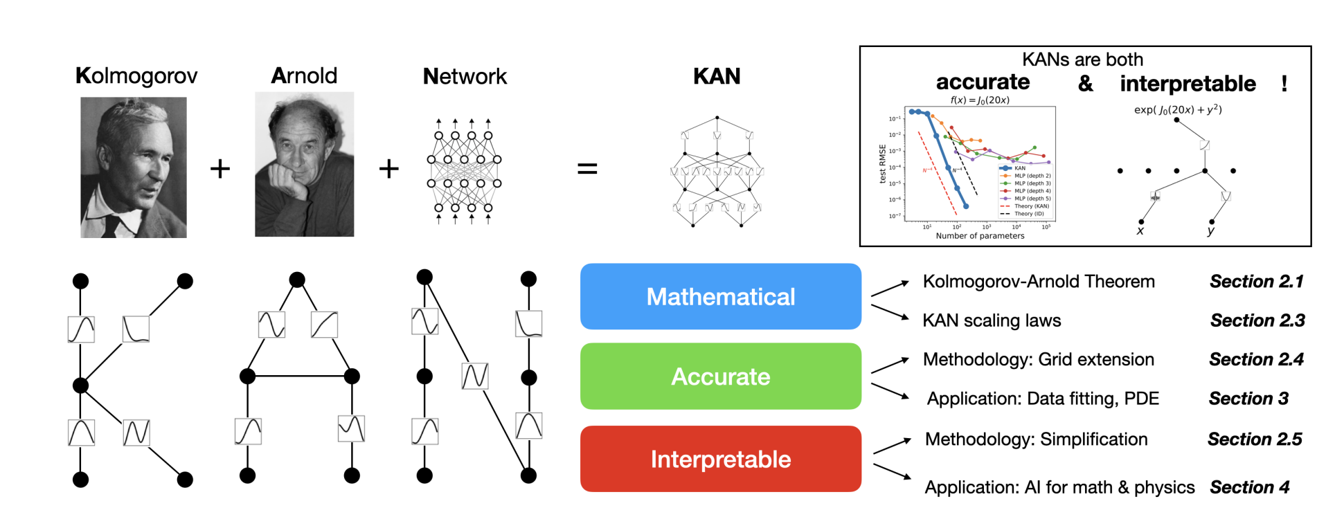
A new machine learning paper dropped by that boldly presents a new path in the deep-learning field. The recent publication on Kolmogorov-Arnold Networks (KANs) is precisely one of those groundbreaking works. Today, we'll try to understand this paper's ideas and fundamental concepts of KANs.

A new machine-learning algorithm, Kolmogorov-Arnold Networks (KANs) promises to be an alternative to Multi-Layer Perceptron. Multi-layer perceptrons (MLPs), or fully-connected feedforward neural networks, are like the foundational blocks of modern deep learning. They're important for tackling complex problems because they're good at approximating curved relationships between input and output data.

To help you understand KANs better, we have added a notebook demo using Paperspace. Paperspace GPUs excel at parallel computing, efficiently handling thousands of simultaneous operations, making them ideal for tasks like deep learning and data analysis. Switching to Paperspace services provides scalable, on-demand access to powerful hardware, eliminating the need for significant upfront investments and maintenance.

But, are KANs the ultimate solution for building models that understand and predict things?

Despite their widespread use, MLPs do have some downsides. For instance, in models like transformers, MLPs use up a lot of the parameters that aren't involved in embedding data. Plus, they're often difficult to understand making them a black box model, compared to other parts of the model, like attention layers, which can make it harder to figure out why they make certain predictions without additional analysis tools.

Why is it considered as an alternative to MLP?

While MLPs are all about fixed activation functions on nodes, KANs flip the script by putting learnable activation functions on the edges. This means each weight parameter in a KAN is replaced by a learnable 1D function, making the network more flexible. Surprisingly, despite this added complexity, KANs often require smaller computation graphs than MLPs. In fact, in some cases, a simpler KAN can outperform a much larger MLP both in accuracy and parameter efficiency, like in solving partial differential equations (PDE).

Other research papers have also attempted to apply this theorem to train machine learning models in the past. However, this particular paper takes a step further by expanding the idea. It introduces a more generalized approach so that we can train neural networks of any size and complexity using backpropagation.

What is KAN?

KANs are based on the Kolmogorov-Arnold representation theorem,

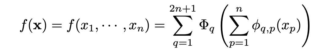
To understand this, let us take an example of a multivariate equation like this,

This is a multivariate function because here, y depends upon x1, x2, ...xn.
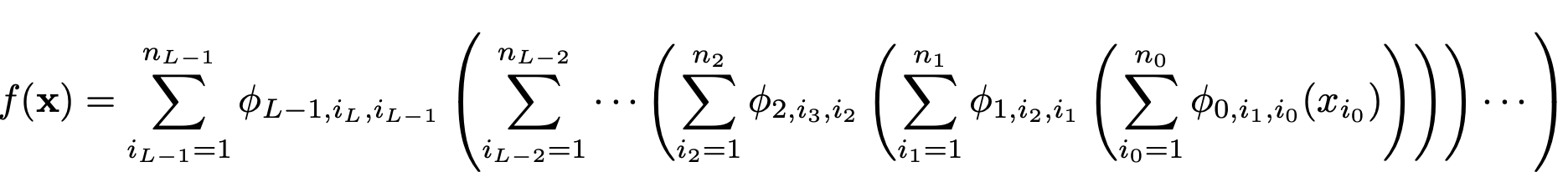
According to the theorem, we can express this as a combination of single-variable functions. This allows us to break down the multivariable equation into several individual equations, each involving one variable and another function of it, and so forth. Then sum up the outputs of all of these functions and pass that sum through yet another univariate function, f as shown here.

Further, instead of making one composition, we do multiple compositions, such as m different compositions and sum them up.

Also, We can rewrite the above equation to,

Overview of the Paper

The paper demonstrated that addition is the only true multivariate function, as every other function can be expressed through a combination of univariate functions and summation. At first glance, this might seem like a breakthrough for machine learning, reducing the challenge of learning high-dimensional functions to mastering a polynomial number of 1D functions.
In simpler terms, it's like saying that even when dealing with a complicated equation or a machine learning task where the outcome depends on many factors, we can break it down into smaller, easier-to-handle parts. We focus on each factor individually, sort of like solving one piece of the puzzle at a time, and then put everything together to solve the bigger problem. So, the main challenge becomes figuring out how to deal with these individual parts, which is where machine learning and techniques like backpropagation step in to help us out.

The original Kolmogorov-Arnold representation equation aligns with a 2-layer KAN having a shape of [n, 2n + 1, 1].

It's worth noting that all operations within this representation are differentiable, enabling us to train KANs using backpropagation.

The above equation shows that the outer sum loops through all of the different compositions from 1 to m. Further, the inner sum loops through each input variable x1 to xn for each outer function q. In matrix form, this can be represented below.

Here, the inner function can be depicted as a matrix filled with various activation functions (denoted as phi). Additionally, we have an input vector (x) with n features, which will traverse through all the activation functions. Please note here that phi represents as the activation function and not the weights. These activation functions are called B-Splines. To add here each of these functions are simple polynomial curves. The curves depend on the input of x.

Visual Representation of KAN

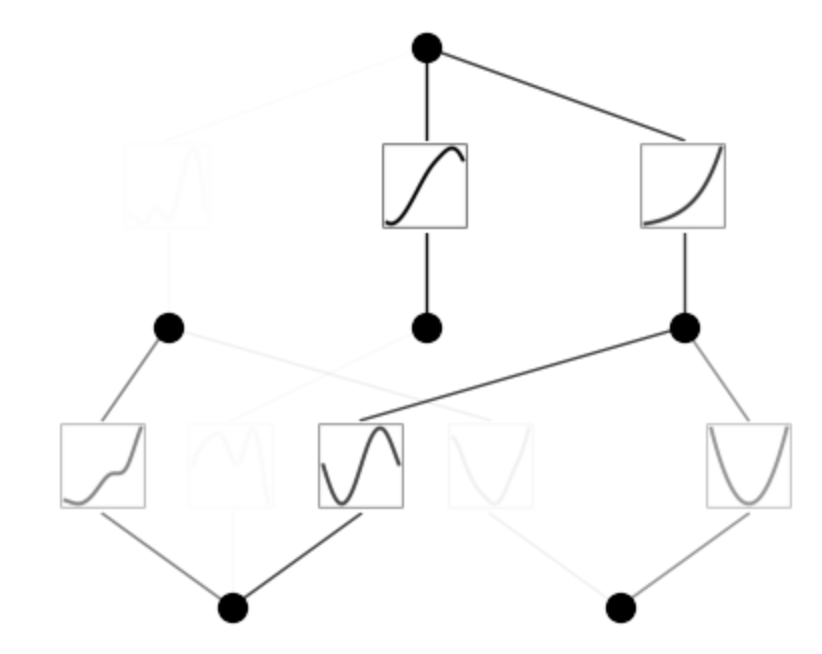
Here is a visual representation of training a 3-layer KAN,

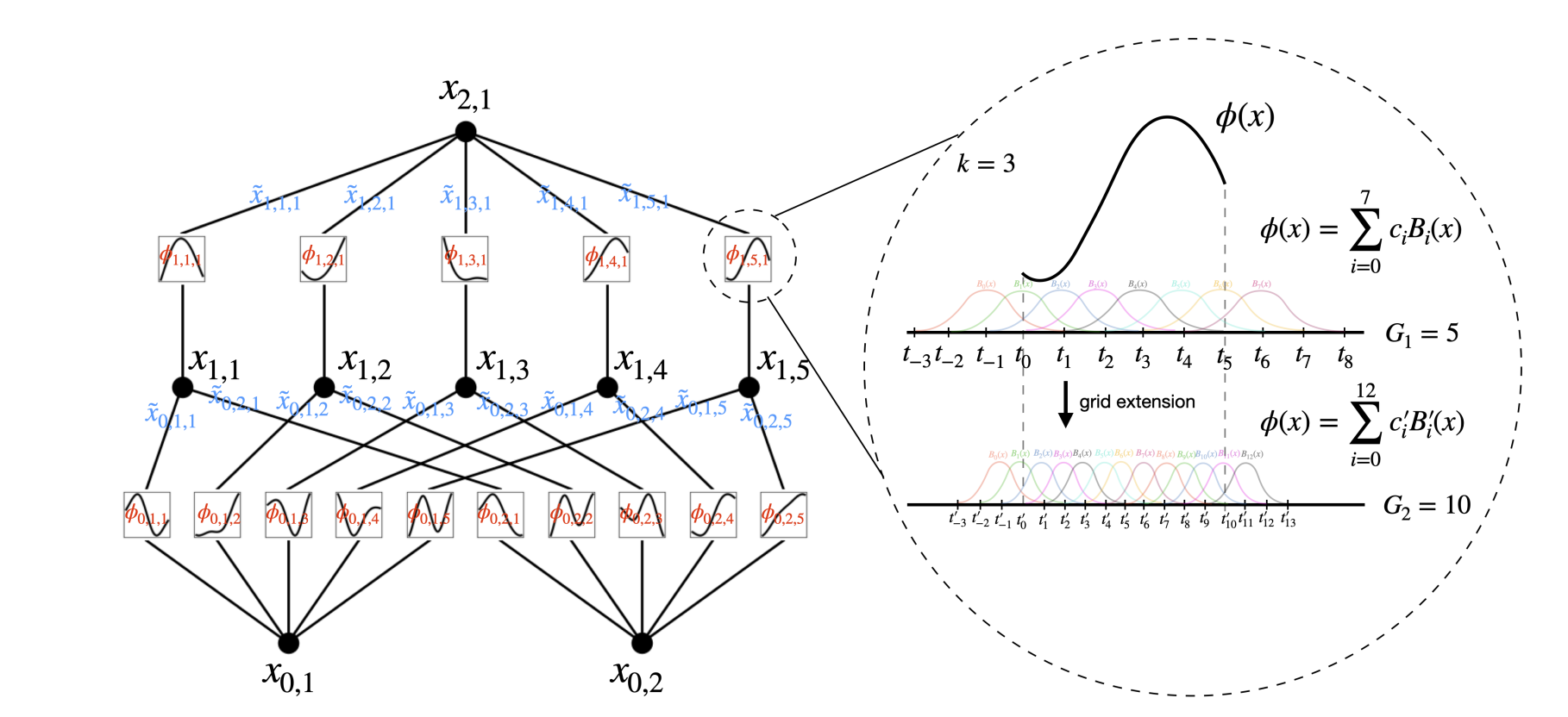
In the given illustration, there are two input features and a first output layer consisting of five nodes. Each output from these nodes undergoes five distinct parameterized univariate activation functions. The resulting activations are then summed to yield the features for each output node. This entire process constitutes a single KAN layer with an input dimension of 2 and an output dimension of 5. Like multi-layer perceptron (MLP), multiple KAN layers can be stacked on top of each other to generate a long, deeper neural network. The output of one layer is the input to the next. Further, like MLPs, the computation graph is fully differentiable, as it relies on differentiable activation functions and summation at the node level, enabling training via backpropagation and gradient descent.

Difference between MLPs and KANs

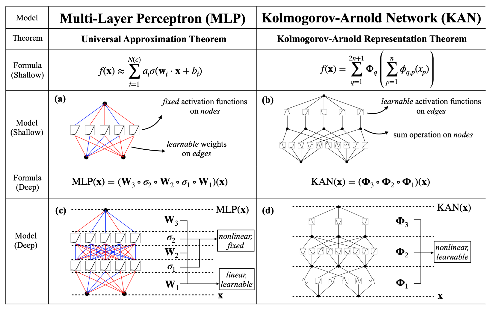
One key differentiator between the two networks is that MLPs place fixed activation functions on the nodes. In contrast, KANs place learnable activation functions along the edges, and the nodes sum it up.

In MLPs, activation functions are parameter-free and perform fixed operations on inputs, while learnable parameters are just linear weights and biases. In contrast, KANs lack linear weight matrices entirely; instead, each weight parameter is substituted with a learnable non-linear activation function.
Also, considering the instability issue with traditional activation functions in neural networks makes training quite challenging. To address this, the authors of KANs employ B-splines, which offer greater stability and bounded behavior.

B-Splines

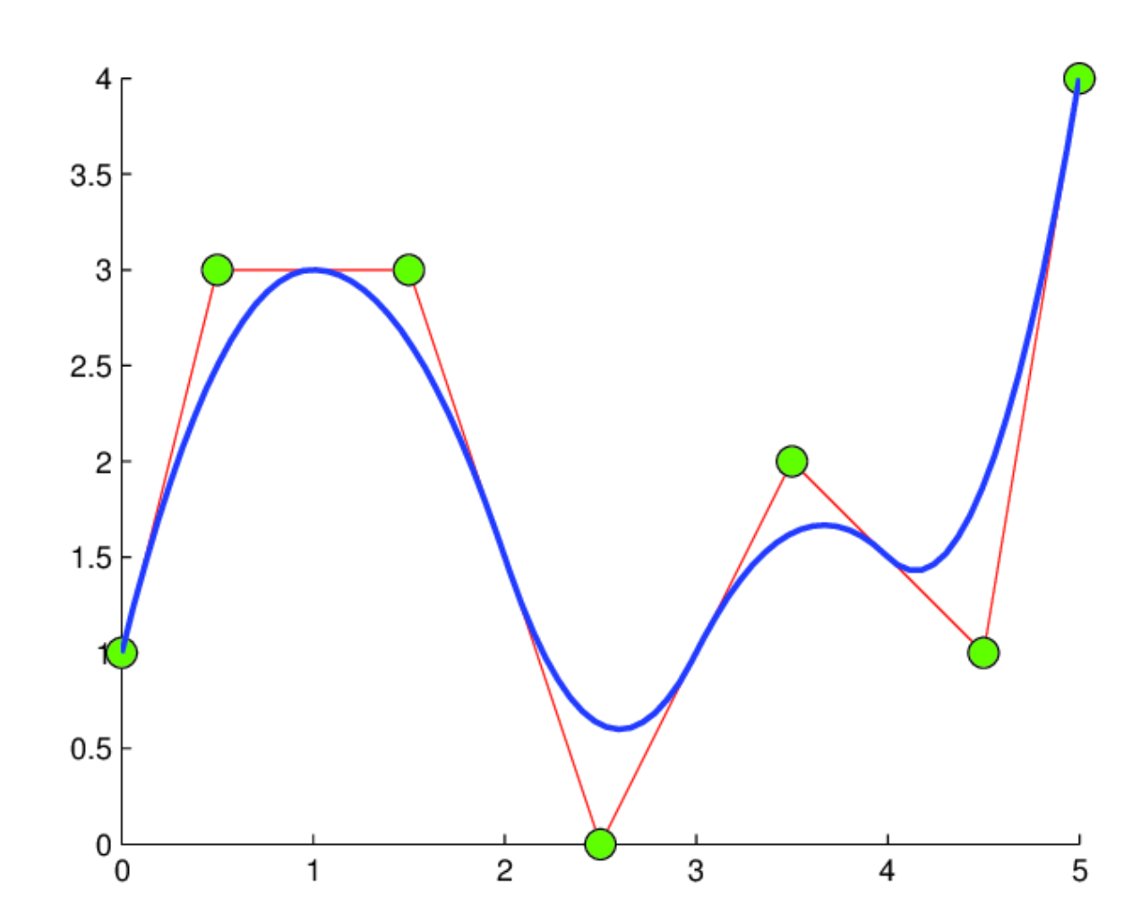
Now, let's understand B-splines briefly. B-splines are essentially curves made up of polynomial segments, each with a specified level of smoothness. Picture each segment as a small curve, where multiple control points influence the shape. Unlike simpler spline curves, which rely on only two control points per segment, B-splines use more, leading to smoother and more adaptable curves.

The magic of B-splines lies in their local impact. Adjusting one control point affects only the nearby section of the curve, leaving the rest undisturbed. This property offers remarkable advantages, especially in maintaining smoothness and facilitating differentiability, which is crucial for effective backpropagation during training.

Training KANs

Backpropagation is a crucial technique for lowering the loss in machine learning. It is crucial for training neural networks by iteratively adjusting their parameters based on observed errors. In KANs, backpropagation is essential for fine-tuning network parameters, including edge weights and coefficients of learnable activation functions.

Training KANs begin with the random initialization of network parameters. The network then undergoes forward and backward passes: input data is fed through the network to generate predictions, which are compared to actual labels to calculate loss. Backpropagation computes gradients of the loss with respect to each parameter using the chain rule of calculus. These gradients guide the parameter updates through methods like gradient descent, stochastic gradient descent, or Adam optimization.

A key challenge in training KANs is ensuring stability and convergence during optimization. Researchers use techniques such as dropout and weight decay for regularization and carefully select optimization algorithms and learning rates to address this. Additionally, batch normalization and layer normalization techniques help stabilize training and accelerate convergence.

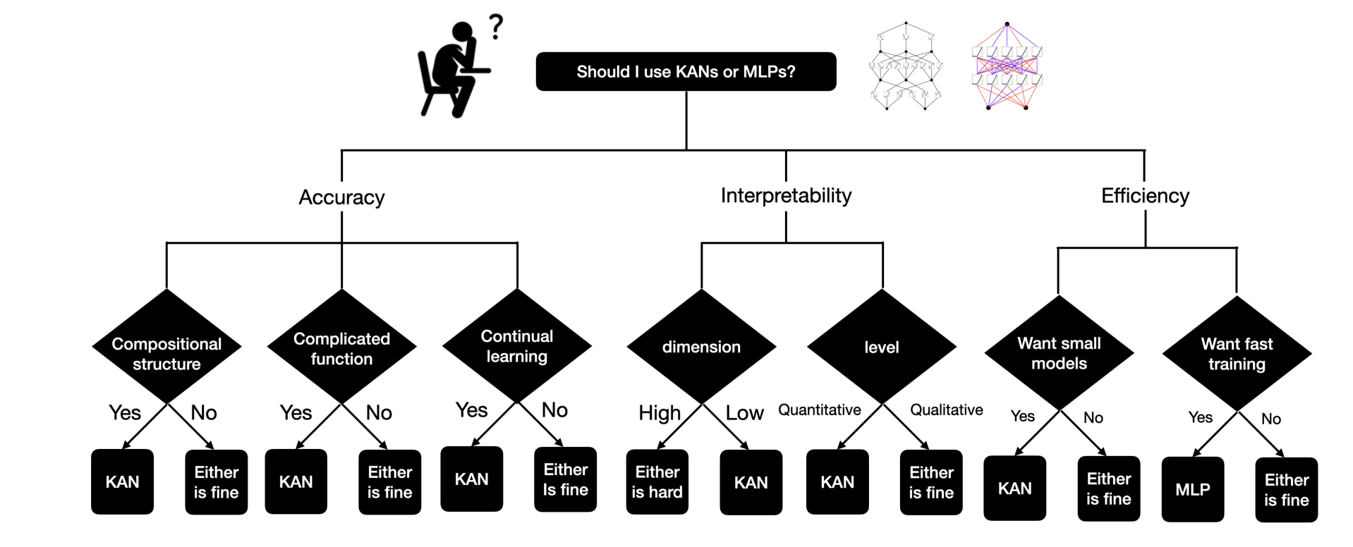
KANs or MLPs?

The main drawback of KANs is their slow training speed, which is about 10 times slower than MLPs with the same number of parameters. However, the research has not yet focused much on optimizing KANs' efficiency, so there is still scope for improvement. If you need fast training, go for MLPs. But if you prioritize interpretability and accuracy, and don't mind slower training, KANs are worth a try.

The key differentiators between MLPs and KANs are:

(i) Activation functions are on edges instead of on nodes,

(ii) Activation functions are learnable instead of fixed.

Advantages of KAN's

• KAN's can learn their activation functions, thus making them more expressive than standard MLPs, and able to learn functions with fewer parameters.
• Further, the paper shows that KANs outperform MLPs using significantly fewer parameters.
• A technique called grid extension allows for fine-tuning KANs by making the spline control grids finer, increasing accuracy without retraining from scratch. This adds more parameters to the model for higher variance and expressiveness.
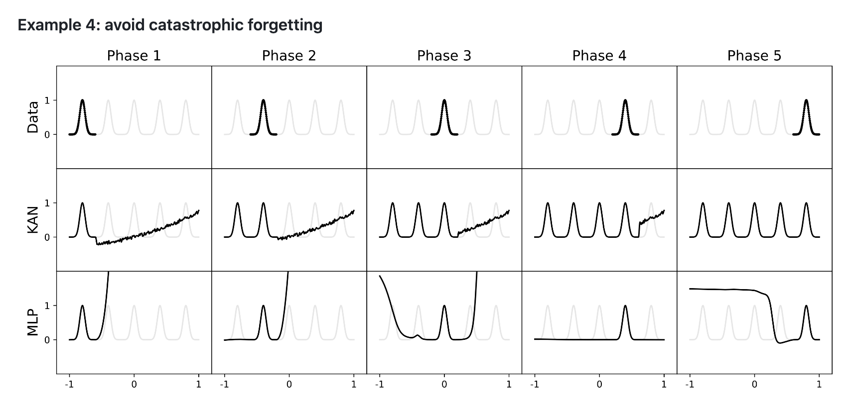
• KANs are less prone to catastrophic forgetting due to B-splines' local control.
  • Catastrophic forgetting occurs when a trained neural network forgets previous training upon fine-tuning with new data.
  • In MLPs, weights change globally, causing the network to forget old data when learning new data.
  • In KANs, adjusting control points of splines affects only local regions, preserving previous training.
• The paper contains many other interesting insights and techniques related to KANs; hence, we highly recommend that our readers read it.

Get KANs working

Install via github:

!pip install git+https://github.com/KindXiaoming/pykan.git

Install via PyPI:

!pip install pykan

Requirements:

# python==3.9.7
matplotlib==3.6.2
numpy==1.24.4
scikit_learn==1.1.3
setuptools==65.5.0
sympy==1.11.1
torch==2.2.2
tqdm==4.66.2

Initialize KAN and create a KAN,

from kan import *
# create a KAN: 2D inputs, 1D output, and 5 hidden neurons. cubic spline (k=3), 5 grid intervals (grid=5).
model = KAN(width=[2,5,1], grid=5, k=3, seed=0)

# create dataset f(x,y) = exp(sin(pi*x)+y^2)
f = lambda x: torch.exp(torch.sin(torch.pi*x[:,[0]]) + x[:,[1]]**2)
dataset = create_dataset(f, n_var=2)
dataset['train_input'].shape, dataset['train_label'].shape

# plot KAN at initialization
model(dataset['train_input']);
model.plot(beta=100)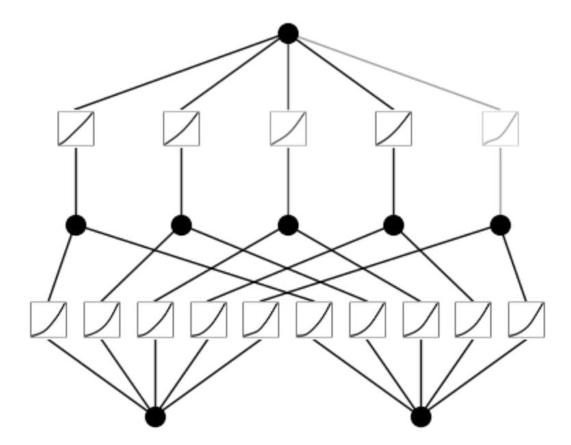

# train the model
model.train(dataset, opt="LBFGS", steps=20, lamb=0.01, lamb_entropy=10.);

model.plot()

model.prune()
model.plot(mask=True)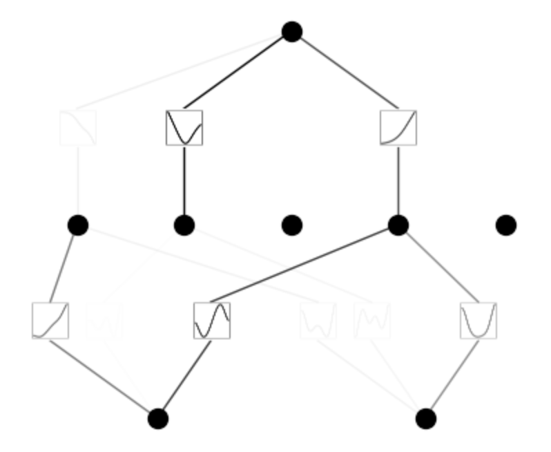

model = model.prune()
model(dataset['train_input'])
model.plot()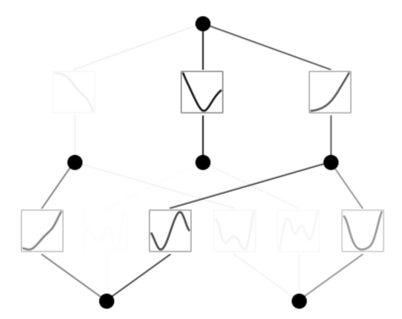

model.train(dataset, opt="LBFGS", steps=50);

train loss: 2.09e-03 | test loss: 2.17e-03 | reg: 1.64e+01 : 100%|██| 50/50 [00:20<00:00, 2.41it/s]

model.plot()

mode = "auto" # "manual"

if mode == "manual":
    # manual mode
    model.fix_symbolic(0,0,0,'sin');
    model.fix_symbolic(0,1,0,'x^2');
    model.fix_symbolic(1,0,0,'exp');
elif mode == "auto":
    # automatic mode
    lib = ['x','x^2','x^3','x^4','exp','log','sqrt','tanh','sin','abs']
    model.auto_symbolic(lib=lib)

fixing (0,0,0) with log, r2=0.9692028164863586
fixing (0,0,1) with tanh, r2=0.6073551774024963
fixing (0,0,2) with sin, r2=0.9998868107795715
fixing (0,1,0) with sin, r2=0.9929550886154175
fixing (0,1,1) with sin, r2=0.8769869804382324
fixing (0,1,2) with x^2, r2=0.9999980926513672
fixing (1,0,0) with tanh, r2=0.902226448059082
fixing (1,1,0) with abs, r2=0.9792929291725159
fixing (1,2,0) with exp, r2=0.9999933242797852

model.train(dataset, opt="LBFGS", steps=50);

train loss: 1.02e-05 | test loss: 1.03e-05 | reg: 1.10e+03 : 100%|██| 50/50 [00:09<00:00, 5.22it/s]

Summary of KANs' Limitations and Future Directions

As per the research we've found that KANs outperform MLPs in scientific tasks like fitting physical equations and solving PDEs. They show promise for complex problems such as Navier-Stokes equations and density functional theory. KANs could also enhance machine learning models, like transformers, potentially creating "kansformers."

KANs excel because they communicate in the "language" of science functions. This makes them ideal for AI-scientist collaboration, enabling easier and more effective interaction between AI and researchers. Instead of aiming for fully automated AI scientists, developing AI that assists scientists by understanding their specific needs and preferences is more practical.

Further, significant concerns need to be addressed before KANs can potentially replace MLPs in machine learning. The main issue is that KANs can't utilize GPU parallel processing, preventing them from taking advantage of the fast-batched matrix multiplications that GPUs offer. This limitation means KANs train very slowly since their different activation functions can't efficiently leverage batch computation or process multiple data points in parallel. Hence, if speed is crucial, MLPs are better. However, if you prioritize interpretability and accuracy and can tolerate slower training, KANs are a good choice.

Additionally, the authors haven't tested KANs on large machine-learning datasets, so it's unclear if they offer any advantage over MLPs in real-world scenarios.

We hope you found this article interesting. We highly recommend checking the resources section for more information on KANs.

Thanks!

Resources

• Original research paper
• Kolmogorov Arnold Networks (KAN) Paper Explained - An exciting new paradigm for Deep Learning?