Don't miss out: Run Stable Diffusion on Free GPUs with Paperspace Gradient with one click
The structure of neural networks is becoming more and more important in research on artificial intelligence modeling for many applications. There have been two opposing structural paradigms developed: feedback (recurrent) neural networks and feed-forward neural networks. In this article, we present an in-depth comparison of both architectures after thoroughly analyzing each. Then, we compare, through some use cases, the performance of each neural network structure.
First, let's start with the basics.
What is a Neural Network ?
The fundamental building block of deep learning, neural networks are renowned for simulating the behavior of the human brain while tackling challenging data-driven issues.
To create the required output, the input data is processed through several layers of artificial neurons that are stacked one on top of the other. Applications range from simple image classification to more critical and complex problems like natural language processing, text production, and other world-related problems.
Elements of Neural Networks
The neurons that make up the neural network architecture replicate the organic behavior of the brain.
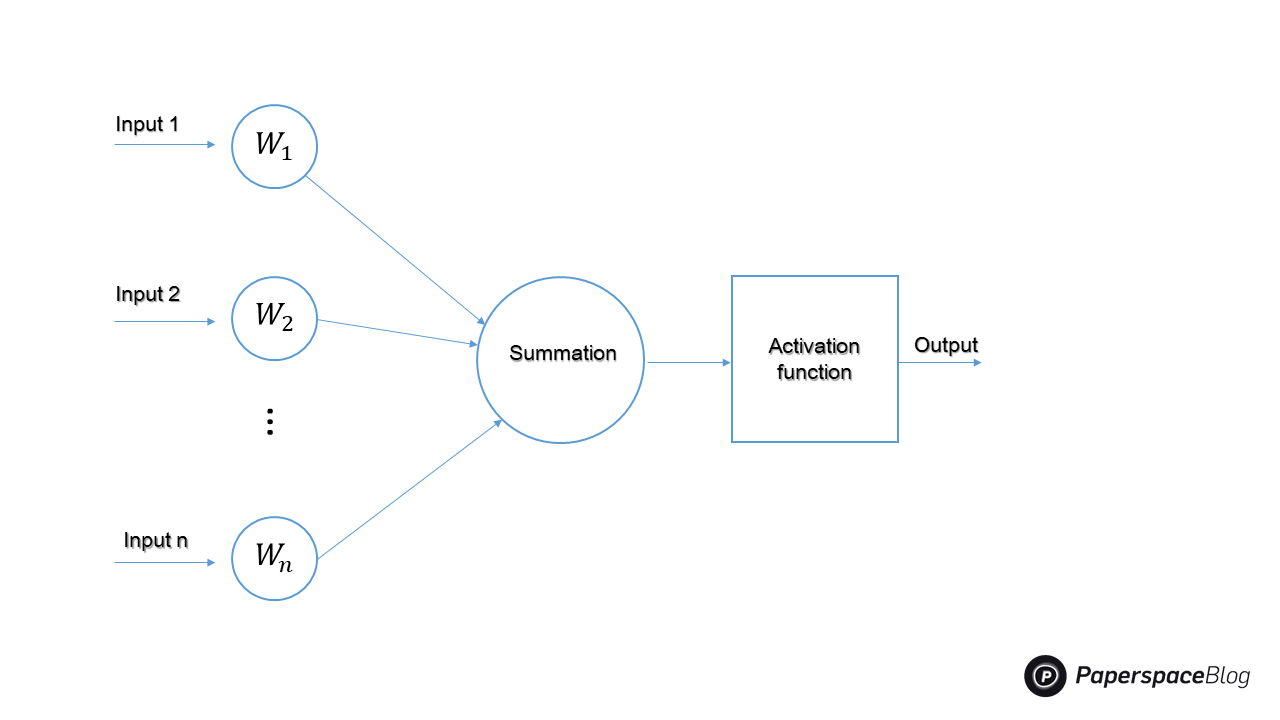
Now, we will define the various components related to the neural network, and show how we can, starting from this basic representation of a neuron, build some of the most complex architectures.
Input
It is the collection of data (i.e features) that are input into the learning model. For instance, an array of current atmospheric measurements can be used as the input for a meteorological prediction model.
Weight
Giving importance to features that help the learning process the most is the primary purpose of using weights. By adding scalar multiplication between the input value and the weight matrix, we can increase the effect of some features while lowering it for others. For instance, the presence of a high pitch note would influence the music genre classification model's choice more than other average pitch notes that are common between genres.
Activation Function
In order to take into account changing linearity with the inputs, the activation function introduces non-linearity into the operation of neurons. Without it, the output would simply be a linear combination of the input values, and the network would not be able to accommodate non-linearity.
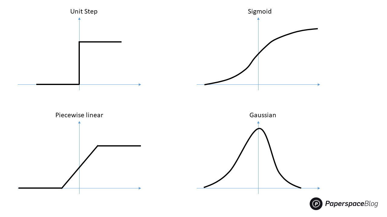
The most commonly used activation functions are: Unit step, sigmoid, piecewise linear, and Gaussian.
Bias
The bias's purpose is to change the value that the activation function generates. Its function is comparable to a constant's in a linear function. So, it's basically a shift for the activation function output.
Layers
An artificial neural network is made of multiple neural layers that are stacked on top of one another. Each layer is made up of several neurons stacked in a row. We distinguish three types of layers: Input, Hidden and Output layer.
Input Layer
The input layer of the model receives the data that we introduce to it from external sources like a images or a numerical vector. It is the only layer that can be seen in the entire design of a neural network that transmits all of the information from the outside world without any processing.
Hidden Layers
The hidden layers are what make deep learning what it is today. They are intermediary layers that do all calculations and extract the features of the data. The search for hidden features in data may comprise many interlinked hidden layers. In image processing, for example, the first hidden layers are often in charge of higher-level functions such as detection of borders, shapes, and boundaries. The later hidden layers, on the other hand, perform more sophisticated tasks, such as classifying or segmenting entire objects.
Output Layer
The final prediction is made by the output layer using data from the preceding hidden layers. It is the layer from which we acquire the final result, hence it is the most important.
In the output layer, classification and regression models typically have a single node. However, it is fully dependent on the nature of the problem at hand and how the model was developed. Some of the most recent models have a two-dimensional output layer. For example, Meta's new Make-A-Scene model that generates images simply from a text at the input.
How these layers work together ?
The input nodes receive data in a form that can be expressed numerically. Each node is assigned a number; the higher the number, the greater the activation. The information is displayed as activation values. The network then spreads this information outward. The activation value is sent from node to node based on connection strengths (weights) to represent inhibition or excitation.
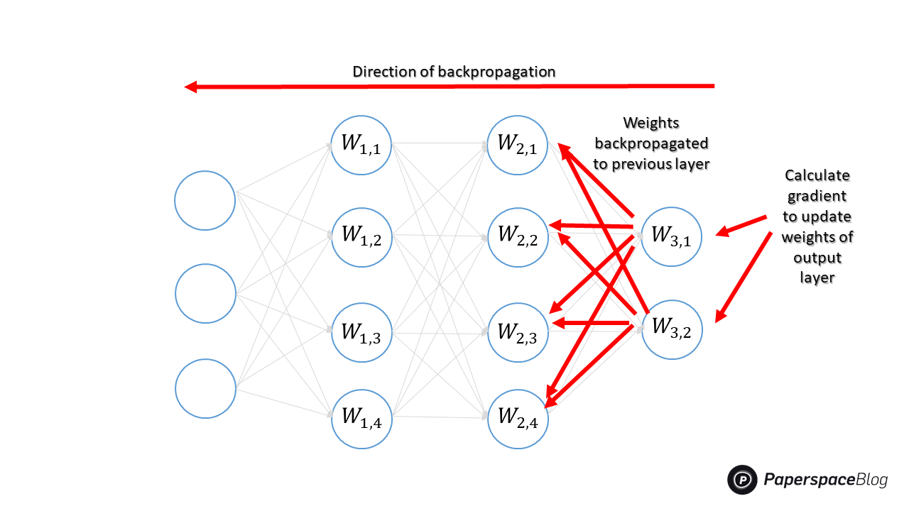
Each node adds the activation values it has received before changing the value in accordance with its activation function. The activation travels via the network's hidden levels before arriving at the output nodes. The input is then meaningfully reflected to the outside world by the output nodes. The error, which is the difference between the projected value and the actual value, is propagated backward by allocating the weights of each node to the proportion of the error that each node is responsible for.
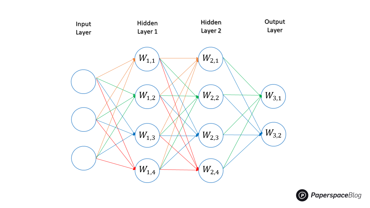
The neural network in the above example comprises an input layer composed of three input nodes, two hidden layers based on four nodes each, and an output layer consisting of two nodes.
Structure of Feed-forward Neural Networks
In a feed-forward network, signals can only move in one direction. These networks are considered non-recurrent network with inputs, outputs, and hidden layers. A layer of processing units receives input data and executes calculations there. Based on a weighted total of its inputs, each processing element performs its computation. The newly derived values are subsequently used as the new input values for the subsequent layer. This process continues until the output has been determined after going through all the layers.
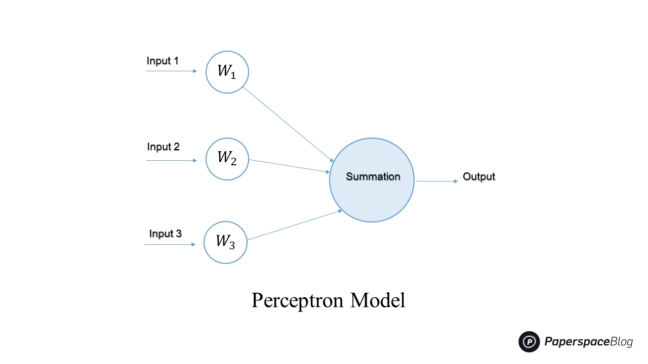
Perceptron (linear and non-linear) and Radial Basis Function networks are examples of feed-forward networks. In fact, a single-layer perceptron network is the most basic type of neural network. It has a single layer of output nodes, and the inputs are fed directly into the outputs via a set of weights. Each node calculates the total of the products of the weights and the inputs. This neural network structure was one of the first and most basic architectures to be built.
Learning is carried out on a multi layer feed-forward neural network using the back-propagation technique. The properties generated for each training sample are stimulated by the inputs. The hidden layer is simultaneously fed the weighted outputs of the input layer. The weighted output of the hidden layer can be used as input for additional hidden layers, etc. The employment of many hidden layers is arbitrary; often, just one is employed for basic networks.
The units making up the output layer use the weighted outputs of the final hidden layer as inputs to spread the network's prediction for given samples. Due to their symbolic biological components, the units in the hidden layers and output layer are depicted as neurodes or as output units.
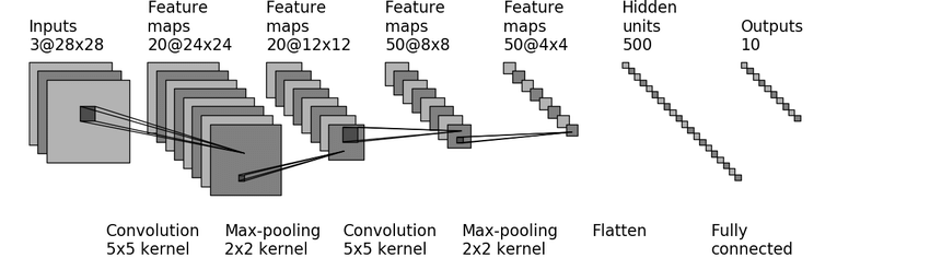
Convolution neural networks (CNNs) are one of the most well-known iterations of the feed-forward architecture. They offer a more scalable technique to image classification and object recognition tasks by using concepts from linear algebra, specifically matrix multiplication, to identify patterns within an image.
Below is an example of a CNN architecture that classifies handwritten digits
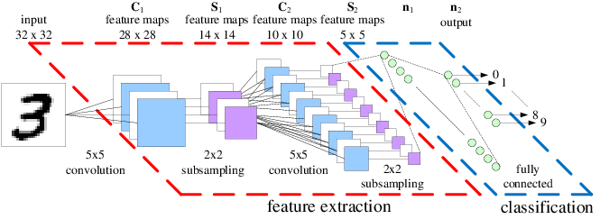
Through the use of pertinent filters, a CNN may effectively capture the spatial and temporal dependencies in an image. Because there are fewer factors to consider and the weights can be reused, the architecture provides a better fitting to the image dataset. In other words, the network may be trained to better comprehend the level of complexity in the image.
How a Feed-forward Neural Network is trained ?
The typical algorithm for this type of network is back-propagation. It is a technique for adjusting a neural network's weights based on the error rate recorded in the previous epoch (i.e., iteration). By properly adjusting the weights, you may lower error rates and improve the model's reliability by broadening its applicability.
The gradient of the loss function for a single weight is calculated by the neural network's back propagation algorithm using the chain rule. In contrast to a native direct calculation, it efficiently computes one layer at a time. Although it computes the gradient, it does not specify how the gradient should be applied. It broadens the scope of the delta rule's computation.
Structure of Feedback Neural Networks
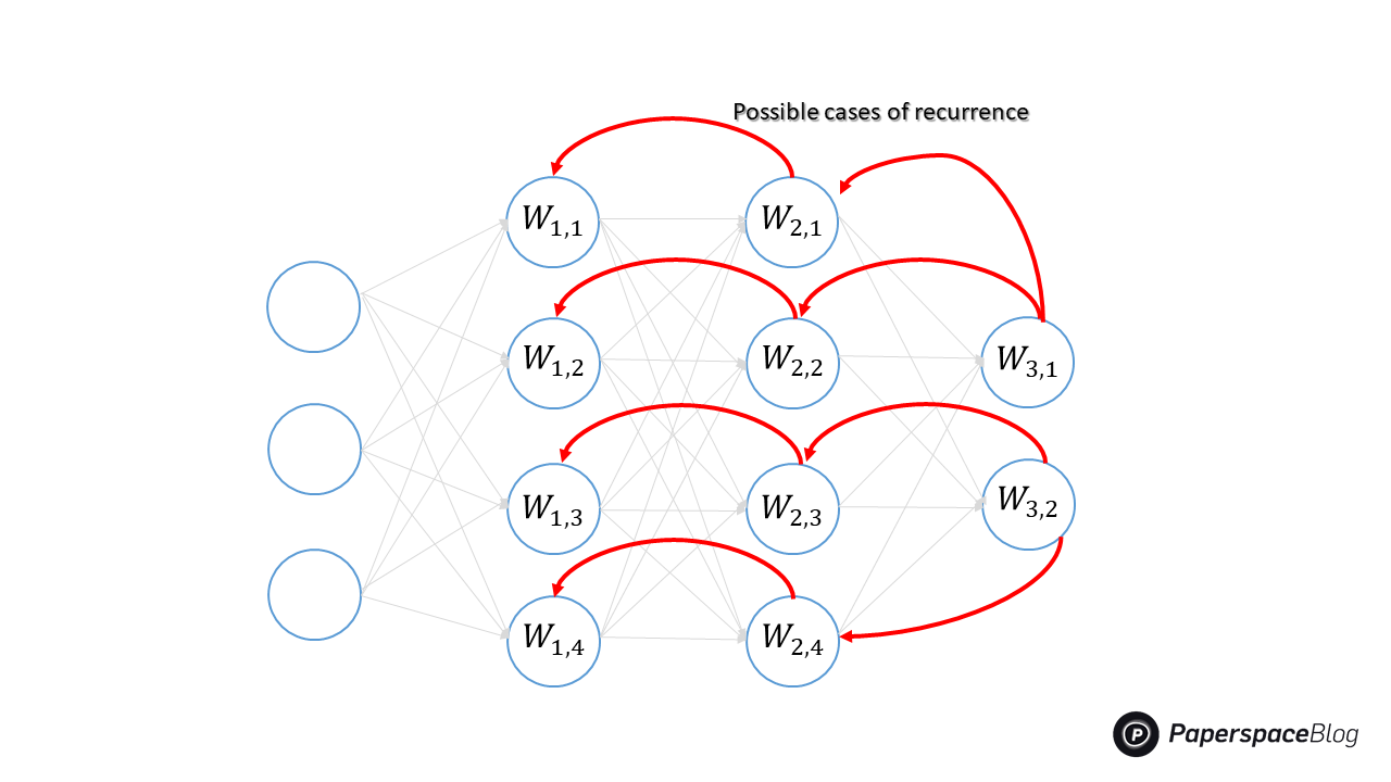
A feed-back network, such as a recurrent neural network (RNN), features feed-back paths, which allow signals to use loops to travel in both directions. Neuronal connections can be made in any way. Since this kind of network contains loops, it transforms into a non-linear dynamic system that evolves during training continually until it achieves an equilibrium state.
In research, RNN are the most prominent type of feed-back networks. They are an artificial neural network that forms connections between nodes into a directed or undirected graph along a temporal sequence. It can display temporal dynamic behavior as a result of this. RNNs may process input sequences of different lengths by using their internal state, which can represent a form of memory. They can therefore be used for applications like speech recognition or handwriting recognition.
How a Feed-back Neural Network is trained ?
Back-propagation through time or BPTT is a common algorithm for this type of networks. It is a gradient-based method for training specific recurrent neural network types. And, it is considered as an expansion of feed-forward networks' back-propagation with an adaptation for the recurrence present in the feed-back networks.
Don't miss out: Run Stable Diffusion on Free GPUs with Paperspace Gradient with one click
CNN vs RNN
As was already mentioned, CNNs are not built like an RNN. RNNs send results back into the network, whereas CNNs are feed-forward neural networks that employ filters and pooling layers.
Application wise, CNNs are frequently employed to model problems involving spatial data, such as images. When processing temporal, sequential data, like text or image sequences, RNNs perform better.
This differences can be grouped in the table below:
| Convolution Neural Networks (CNNs) | Recurrent Neural Networks (RNNs) | |
|---|---|---|
| Architecture | Feed-forward neural network | Feed-back neural network |
| Layout | Multiple layers of nodes including convolutional layers |
Information flows in different directions, simulating a memory effect |
| Data type | Image data | Sequence data |
| Input/Output | The size of the input and output are fixed (i.e input image with fixed size and outputs the classification) |
The size of the input and output may vary (i.e receiving different texts and generating different translations for example) |
| Use cases | Image classification, recognition, medical imagery, image analysis, face detection |
Text translation, natural language processing, language translation, sentiment analysis |
| Drawbacks | Large training data | Slow and complex training procedures |
| Description | CNN employs neuronal connection patterns. And, they are inspired by the arrangement of the individual neurons in the animal visual cortex, which allows them to respond to overlapping areas of the visual field. | Time-series information is used by recurrent neural networks. For instance, a user's previous words could influence the model prediction on what he can says next. |
Architecture examples
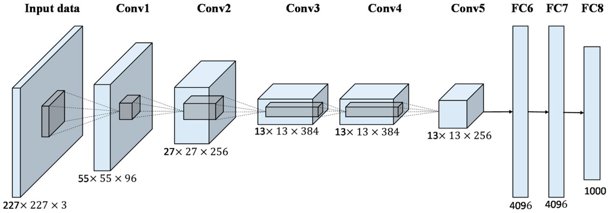
AlexNet
A Convolutional Neural Network (CNN) architecture known as AlexNet was created by Alex Krizhevsky. Eight layers made up AlexNet; the first five were convolutional layers, some of them were followed by max-pooling layers, and the final three were fully connected layers. It made use of the non-saturating ReLU activation function, which outperformed tanh and sigmoid in terms of training efficiency. Considered to be one of the most influential studies in computer vision, AlexNet sparked the publication of numerous further research that used CNNs and GPUs to speed up deep learning. In fact, according to F, the AlexNet publication has received more than 69,000 citations as of 2022.
LeNet
Yann LeCun suggested the convolutional neural network topology known as LeNet. One of the first convolutional neural networks, LeNet-5, aided in the advancement of deep learning. LeNet, a prototype of the first convolutional neural network, possesses the fundamental components of a convolutional neural network, including the convolutional layer, pooling layer, and fully connection layer, providing the groundwork for its future advancement. LeNet-5 is composed of seven layers, as depicted in the figure.
Long short-term memory (LSTM)
LSTM network are one of the prominent examples of RNNs. These architectures can analyze complete data sequences in addition to single data points. For instance, LSTM can be used to perform tasks like unsegmented handwriting identification, speech recognition, language translation and robot control.
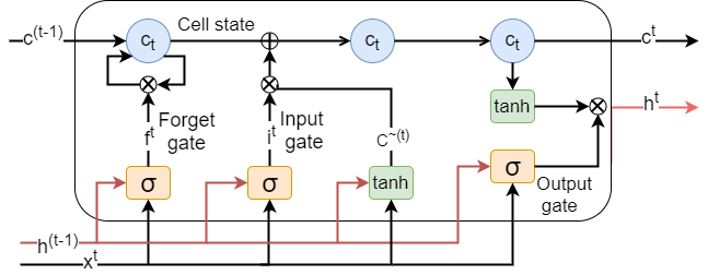
LSTM networks are constructed from cells (see figure above), the fundamental components of an LSTM cell are generally : forget gate, input gate, output gate and a cell state.
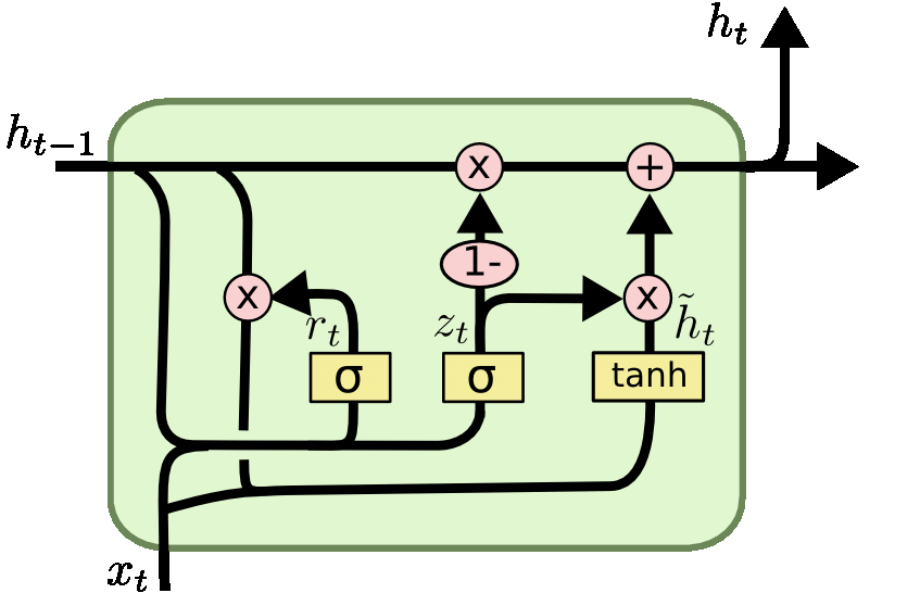
Gated recurrent units (GRU)
This RNN derivative is comparable to LSTMs since it attempts to solve the short-term memory issue that characterizes RNN models. The GRU has fewer parameters than an LSTM because it doesn't have an output gate, but it is similar to an LSTM with a forget gate. It was discovered that GRU and LSTM performed similarly on some music modeling, speech signal modeling, and natural language processing tasks. GRUs have demonstrated superior performance on several smaller, less frequent datasets.
Use cases
Depending on the application, a feed-forward structure may work better for some models while a feed-back design may perform effectively for others. Here are a few instances where choosing one architecture over another was preferable.
Forecasting currency exchange rates
In a research for modeling the Japanese yen exchange rates, and despite being extremely straightforward and simple to apply, results for out of sample data demonstrate that the feed-forward model is reasonably accurate in predicting both price levels and price direction. In fact, the feed-forward model outperformed the recurrent network forecast performance. This may be due to the fact that feed-back models, which frequently experience confusion or instability, must transmit data both from back to forward and forward to back.
Recognition of Partially Occluded Objects
There is a widespread perception that feed-forward processing is used in object identification. Recurrent top-down connections for occluded stimuli may be able to reconstruct lost information in input images. The Frankfurt Institute for Advanced Studies' AI researchers looked into this topic. They have demonstrated that for occluded object detection, recurrent neural network architectures exhibit notable performance improvements. The same findings were reported in a different article in the Journal of Cognitive Neuroscience. The experiment and model simulations that go along with it, carried out by the authors, highlight the limitations of feed-forward vision and argue that object recognition is actually a highly interactive, dynamic process that relies on the cooperation of several brain areas.
Image classification
In some instances, simple feed-forward architectures outperform recurrent networks when combined with appropriate training approaches. For instance, ResMLP, an architecture for image classification that is solely based on multi-layer perceptrons. A research project showed the performance of such structure when used with data-efficient training. It was demonstrated that a straightforward residual architecture with residual blocks made up of a feed-forward network with a single hidden layer and a linear patch interaction layer can perform surprisingly well on ImageNet classification benchmarks if used with a modern training method like the ones introduced for transformer-based architectures.
Text classification
RNNs are the most successful models for text classification problems, as was previously discussed. Three distinct information-sharing strategies were proposed in a study to represent text with shared and task-specific layers. All of these tasks are jointly trained over the entire network. The proposed RNN models showed a high performance for text classification, according to experiments on four benchmark text classification tasks.
An LSTM-based sentiment categorization method for text data was put forth in another paper. This LSTM technique demonstrated performance for sentiment categorization with an accuracy rate of 85%, which is considered a high accuracy for sentiment analysis models.
Tutorials
In Paperspace, many tutorials were published for both CNNs and RNNs, we propose a brief selection in this list to get you started:
 Nanda Kishor M Pai
In this tutorial, we used the PyTorch implementation of a CNN structure to localize the position of a given object inside an image at the input.
Ahmed Fawzy Gad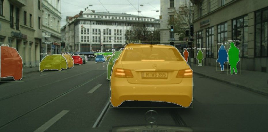
In this post, we propose an implementation of R-CNN, using the library Keras, to make an object detection model.
Samhita Alla
While in this article, we implement using Keras a model called Seq2Seq, which is a RNN model used for text summarization.
Samhita Alla
Then, in this implementation of a Bidirectional RNN, we made a sentiment analysis model using the library Keras.
Conclusion
To put it simply, different tools are required to solve various challenges. It's crucial to understand and describe the problem you're trying to tackle when you first begin using machine learning. It takes a lot of practice to become competent enough to construct something on your own, therefore increasing knowledge in this area will facilitate implementation procedures.
In this post, we looked at the differences between feed-forward and feed-back neural network topologies. Then we explored two examples of these architectures that have moved the field of AI forward: convolutional neural networks (CNNs) and recurrent neural networks (RNNs). We then, gave examples of each structure along with real world use cases.
Resources
https://link.springer.com/article/10.1007/BF00868008
https://arxiv.org/pdf/2104.10615.pdf
https://dl.acm.org/doi/10.1162/jocn_a_00282
https://arxiv.org/pdf/2105.03404.pdf
https://proceedings.neurips.cc/paper/2012/file/c399862d3b9d6b76c8436e924a68c45b-Paper.pdf
https://www.ijcai.org/Proceedings/16/Papers/408.pdf
https://www.ijert.org/research/text-based-sentiment-analysis-using-lstm-IJERTV9IS050290.pdf