End-to-End Recommender System with Gradient - Part 4: Tuning the Model for Best Performance

Introduction to Part 4

In the fourth part of this six-part series, we will improve the result from the model in Part 3 by tuning some of its hyperparameters and demonstrate how the training process can be done in Gradient Workflows.

Series parts

Part 1: Posing a business problem
Part 2: Preparing the data
Part 3: Building a TensorFlow model
Part 4: Tuning the model for best performance
Part 5: Deploying the model into production
Part 6: Summary, conclusions, and next steps

Accompanying material

• The main location for accompanying material to this blog series is the GitHub repository at https://github.com/gradient-ai/Deep-Learning-Recommender-TF .
• This contains the notebook for the project, deep_learning_recommender_tf.ipynb, which can be run in Gradient Notebooks or the JupyterLab interface, and 3 files for the Gradient Workflow: workflow_train_model.py, workflow-train-model.yaml and workflow-deploy-model.yaml.
• The repo is designed to be able to be used and followed along without having to refer to the blog series, and vice versa, but they compliment each other.

NOTE

Model deployment support in the Gradient product on public clusters and from Workflows is currently pending, expected in 2021 Q4. Therefore section 5 of the Notebook deep_learning_recommender_tf.ipynb on model deployment is shown but will not yet run.

Tuning in Gradient

In Part 3, we showed how to build and train a basic recommender model. Now we will tune some of the hyperparameters to improve its performance.

While tuning could be done entirely in a Notebook, Gradient also allows hyperparameter tuning as part of Gradient Workflows.

The advantage of Gradient Workflows is that we can integrate with Git, Docker containers, and the full definition of run parameters via YAML to enable versioned and reproducible experiments.

Once we have experiments of this nature, we can use Gradient's modern MLOps stack (which includes CI/CD, microservices, Kubernetes, and so on) to deploy models into production.

What we mean when we talk about MLOps

CI/CD refers to continuous integration – in which versions of code and other objects are merged correctly – and continuous deployment – in which software is rapidly deployed and regularly updated in an automated manner.

While CI/CD has become widespread in software development, the concept needs to adapt to fit the ML use case because ML models deal with changing data and are therefore not fixed along the same parameters.

Kubernetes has become the de facto container orchestration system used by machine learning teams to assign compute resources, but is generally regarded as difficult for non-engineer data scientists to configure.

A particular strength of Gradient is that what works for the single node case is straightforwardly extended to the multinode case. The user can simply add the appropriate extra settings to the single node case to specify multinode requirements and Gradient will handle the distribution. We discuss these possibilities in more detail at the end of Part 6.

Implementation of tuning

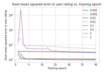
In this tutorial we will do some basic tuning using TensorFlow to demonstrate capabilities. We will vary the learning rate on a logarithmic scale and then zoom in to a linear scale around the best value from the logarithmic scale. We will also train the model for more epochs, and add L2 regularization.

When using the TensorFlow subclassing API with the full model classes, part of what needs to be specified is how and what hyperparameters are passed to the model. Since our tuning is relatively simple, we add the regularizer to the model code, and pass in the number of epochs and learning rate to the .compile and .fit steps.

The model tuning loop looks like this:

learning_rates_logarithmic = [0.001, 0.01, 0.1, 1]
epochs = 30
histories_tr = {}
...
for val in learning_rates_logarithmic:
    print('Learning rate = {}'.format(val))
    model_tr = MovielensModelTunedRanking()
    model_tr.compile(optimizer=tf.keras.optimizers.Adagrad(learning_rate=val))
    lr = str(val)
    histories_tr[lr] = model_tr.fit(cached_train, epochs=epochs, validation_data=cached_validation)

For more extensive tuning, more complex loops can be written. It's also possible to use additional libraries such as HParams or to use smart-search/AutoML to search larger spaces more efficiently than grid search.

For the purposes of this series, our tuning is simple. We can make a single inline plot of its values using Matplotlib:

For more complex hyperparameter sets or other visualizations, Gradient allows intermediate stages on longer tuning runs to be saved via TensorFlow callbacks.

We find that a learning rate of 0.1 is best, and zooming in, it remains best when a linear grid is used too. Besides the learning rate, we also ran the model for more epochs, and the result is the mean squared error in the prediction is improved from 1.11 to 1.06.

This is not a huge improvement, but it is significant. It achieves our aim of showing model tuning that improves the result. There are many other hyperparameters that can be tuned (the author tried a few), but simple changes like varying the optimizer or the layer sizes and numbers didn't make a large difference.

The best way to improve from the results here is to incorporate more sophisticated architectural components of a full recommender system, as shown for example in the series of TFRS tutorials.

The winning strategy is to integrate concepts such as cross-features and adding the time series seasonality that we mentioned but didn't implement.

All of these possibilities are just longer versions of models using the same fully generalized TensorFlow subclassed API interface that we have shown here -- so clearly they could be implemented and deployed in the Gradient ecosystem if the user so desired.

Now that we have a model that is trained and has been tuned to perform well enough for our purposes, the next step is to deploy it into production.

Training the final model in Workflows

In the above, we did the tuning from the notebook, and the results and versioning are somewhat ad hoc.

A more rigorous approach is provided by Gradient Workflows, where the data, model, and versions of the inputs and outputs are all fixed for a given run.

Rather than repeat the whole tuning here, we just show the Workflow equivalent of training the final model. The relevant portions of the notebook code are repeated in a Python .py script, and the workflow is specified in a YAML file.

Here the Workflow is called from the Notebook, using the Gradient SDK, but it can also be called from the command line without requiring a notebook to be used.

YAML will be less familiar to many users, but YAML syntax (or something like it) is necessary to specify the workflow to the required level of precision to make it production-grade.

We provide various examples of how to use it (and Workflows) in the Gradient documentation. In particular, there is a page Using YAML for data science which addresses several issues likely to come up for non-YAML-experts doing data science.

For training our final model, the .py script repeats the data preparation, model class definition, and model training portions of the notebook. The YAML file for training the model looks like this:

...

defaults:
  resources:
    instance-type: P4000
  env:
    PAPERSPACE_API_KEY: secret:api_key_recommender

jobs:

...

  CloneRecRepo:
    outputs:
      repoRec:
        type: volume
    uses: git-checkout@v1
    with:
      url: https://github.com/gradient-ai/Deep-Learning-Recommender-TF

...

  RecommenderTrain:
    needs:
      - CloneRecRepo
    inputs:
      repoRec: CloneRecRepo.outputs.repoRec
    env:
      HP_FINAL_EPOCHS: '50'
      HP_FINAL_LR: '0.1'
    outputs:
      trainedRecommender:
        type: dataset
        with:
          ref: recommender
    uses: script@v1
    with:
      script: |-
        cp -R /inputs/repoRec /Deep-Learning-Recommender-TF
        cd /Deep-Learning-Recommender-TF
        python workflow_train_model.py
      image: tensorflow/tensorflow:2.4.1-jupyter
      

We can see that it runs two jobs, CloneRecRepo and RecommenderTrain.

CloneRecRepo gets the specified version of the GitHub repository for this project, here the default of the current master branch, and outputs it as a mounted volume.

In this case, the repo is public, so no credentials (stored in Gradient as Secrets) need to be supplied to clone it. The uses: line specifies a Gradient Action, which is a particular procedure such as cloning a repo or running a command in a container. Gradient Actions can run in parallel.

RecommenderTrain then uses the repo in the mounted volume to train the model and output it to a versioned set of files under trainedRecommender.

We specify that we require the CloneRecRepo job to have completed successfully using needs.

The Gradient Actions script@v1 allows a set of commands to then be run, the main one being our training script, workflow_train_model.py. The script is run on the specified Docker container, tensorflow/tensorflow:2.4.1-jupyter, on Gradient's Kubernetes-managed infrastructure.

The model hyperparameters (or in general any arguments) are passed to the script as environment variables via the env: field.

(The syntax for output is slightly confusing for the RecommenderTrain job since the set of files containing the model are referred to in Gradient as a "dataset." This name may change in future. It is also necessary to copy the repo from the /inputs directory to a working directory because /inputs is read-only. This can also be improved upon, and note that the dataset, which may contain much larger files, does not have to be copied.)

When the training is run, we can see the details of the Workflow in Gradient's GUI:

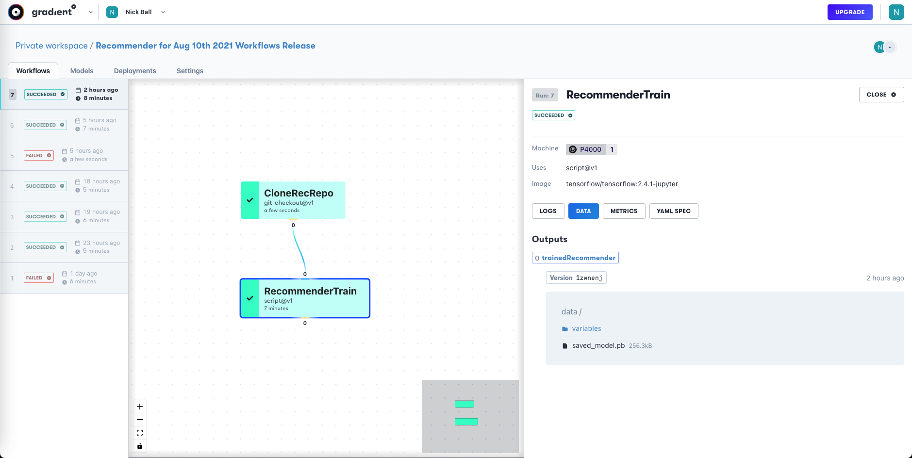
Workflow jobs are shown as a directed acyclic graph (DAG), and the YAML, outputs, and versions can be viewed. Our output is a trained model from the RecommenderTrain job.

The output model is the same as the one we trained above using the notebook.

For full details of the YAML and Workflows, see the Gradient documentation. The .py and YAML files are available in the project GitHub repository as workflow_train_model.py and workflow-train-model.yaml.

Notebooks versus Workflows

The ideal interplay between running a data science project from a notebook, and using a more IDE-based approach with Python scripts is a generic one in the data science and MLOps communities that has not yet been resolved.

There are good reasons for the use of both interfaces at various stages, but the transition from one to the other, typically when going from an exploratory phase to a production phase of a project, can involve code being duplicated or rewritten.

Since Paperspace's products contain the necessary compute hardware, and both the notebook and IDE approaches, Gradient is well-positioned to enable both approaches now and in the future.

Next

In Part 5 of the series - Deploying the model into production, we will show how to deploy the model using Gradient Workflows, and its integration with TensorFlow Serving.