Ensembling Neural Network Models With Tensorflow

Model ensembling is a common practice in machine learning to improve the performance and generalizability of models.  It can be simply described as the technique of combining multiple models in diverse ways to improve performance on a single problem.

The major merits of model ensembling include its ability to improve the performance, robustness and generalization of machine learning models on unseen data.

Tree-based algorithms are particularly known to perform better for certain tasks due to their ability to utilize the ensembling of multiple trees to improve the model's overall performance.

The ensemble members ( i.e models that are combined to a single model or prediction) are combined using diverse aggregation techniques such as simple or weighted averaging to other advanced techniques such as bagging, stacking or boosting.

In contrast to classical algorithms, it's not a common for multiple neural network models to be ensembled for a single task. This is mostly because single models are often enough to map the relationship between features and targets and ensembling multiple neural networks might complicate the model for smaller tasks and lead to overfitting of the model. It's most common for practitioners to increase the size of a single neural network model to properly fit the data than ensemble multiple neural network models into one.

However, for larger tasks, ensembling multiple neural networks, especially ones trained on similar problems, could prove quite useful and improve the performance of the final model and its ability to generalize on broader use cases.

Oftentimes, practitioners try out multiple models with different configurations to select the best-performing model for a problem. Neural network ensembling offers the option of utilizing the information of the different models to develop a more balanced and efficient model.

For example, combining multiple network models that were trained on a particular dataset (such as the Imagenet dataset) could prove useful to improve the performance of a model being trained on a dataset with similar classes. The different information learned by the models could be combined through model ensembling to improve the model's overall performance and robustness of an aggregated model. Before ensembling such models, it is important to train and fine-tune the ensemble members to ensure that each model contributes relevant information to the final model.

The Tensorflow API provides certain techniques for aggregating multiple network models using built-in network layers or by building custom layers.

In this tutorial, we ensemble custom and pre-trained network models that are trained on similar datasets using custom and built-in Tensorflow layers to approach an image classification problem. We would ensemble our models using concatenation, average and weighted average ensembling methods.

This aims to serve as a template of different techniques for combining multiple network models in your projects.

The Dataset

Our use case is an image classification of natural images. We would be using the Natural Images Dataset which contains 6899 images of natural images representing 8 classes. The represented classes in the dataset are aeroplane, car, cat, dog, fruit, motorbike and person.

Our aim is to develop a neural network model that is capable of identifying images belonging to the different classes and accurately classifying new images of each class.

Workflow

We would develop three different models for our task and then ensemble using different methods. It is important to configure our models to provide relevant information to our final model.

Seed the environment for reproducibility and preview some of the images in the dataset representing each class.

# Seed environment 
seed_value = 1 # seed value 

# Set`PYTHONHASHSEED` environment variable at a fixed value 
import os os.environ['PYTHONHASHSEED']=str(seed_value) 

# Set the `python` built-in pseudo-random generator at a fixed value 
import random 
random.seed = seed_value 

# Set the `numpy` pseudo-random generator at a fixed value 
import numpy as np 
np.random.seed = seed_value 

# Set the `tensorflow` pseudo-random generator at a fixed value import tensorflow as tf tf.seed = seed_value

Set the data configurations and get the classes

# set configs 
base_path = './natural_images' 
target_size = (224,224,3) 

# define shape for all images # get classes classes = os.listdir(base_path) print(classes)

Plot Sample images of the dataset

# plot sample images 

import matplotlib.pyplot as plt
import cv2

f, axes = plt.subplots(2, 4, sharex=True, sharey=True, figsize = (16,7))

for ax, label in zip(axes.ravel(), classes):
    img = np.random.choice(os.listdir(os.path.join(base_path, label)))
    img = cv2.imread(os.path.join(base_path, label, img))
    img = cv2.resize(img, target_size[:2])
    ax.imshow(cv2.cvtColor(img, cv2.COLOR_BGRA2RGB))
    ax.set_title(label)
    ax.axis(False)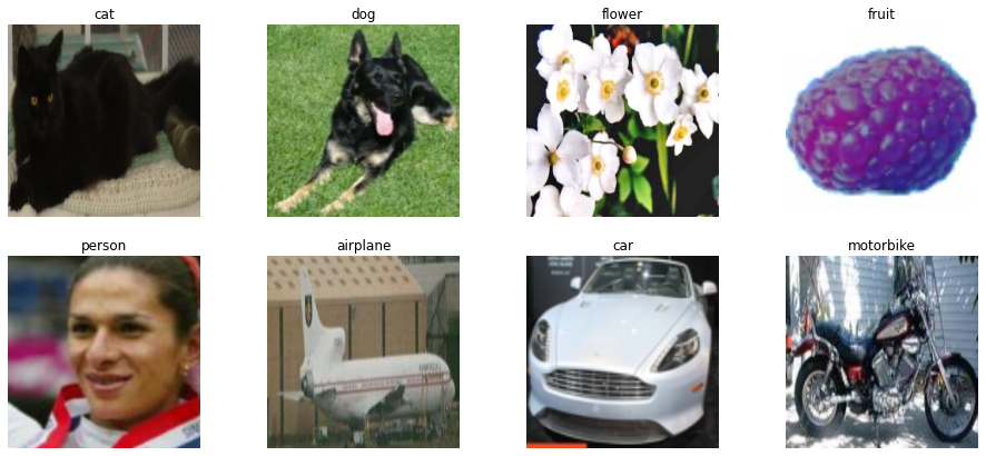

‌Load the images.

We load the images in batches using the Keras Image Generator and specify a validation split to split the dataset into training and validation splits.

We also apply random image augmentation to expand the training dataset in order to improve the performance of the model and its ability to generalize.

from keras.preprocessing.image import ImageDataGenerator

batch_size = 32

datagen = ImageDataGenerator(rescale=1./255,
                                   rotation_range=20,
                                   shear_range=0.2,
                                   zoom_range=0.2,
                                   width_shift_range = 0.2,
                                   height_shift_range = 0.2,
                                   vertical_flip = True,
                                   validation_split=0.25)

train_gen = datagen.flow_from_directory(base_path,
                                               target_size=target_size[:2],
                                               batch_size=batch_size,
                                               class_mode='categorical',
                                               subset='training')
val_gen =  datagen.flow_from_directory(base_path,
                                               target_size=target_size[:2],
                                               batch_size=batch_size,
                                               class_mode='categorical',
                                               subset='validation',
                                               shuffle=False)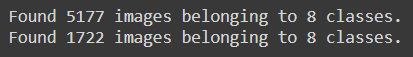

1. Build and train a custom model.‌

For our first model, we build a custom model using the Tensorflow functional method

# Build model 
input = Input(shape= target_size) 

x = Conv2D(filters=32, kernel_size=(3,3), activation='relu')(input) 
x = MaxPool2D(2,2)(x) 

x = Conv2D(filters=64, kernel_size=(3,3), activation='relu')(x) 
x = MaxPool2D(2,2)(x) 

x = Conv2D(filters=128, kernel_size=(3,3), activation='relu')(x) 
x = MaxPool2D(2,2)(x) 

x = Conv2D(filters=256, kernel_size=(3,3), activation='relu')(x) 
x = MaxPool2D(2,2)(x) 

x = Dropout(0.25)(x) 
x = Flatten()(x) 
x = Dense(units=128, activation='relu')(x) 
x = Dense(units=64, activation='relu')(x) 
output = Dense(units=8, activation='softmax')(x) 

custom_model  = Model(input, output, name= 'Custom_Model')

Next, we compile the custom model and initialize the callbacks to monitor and control training. For our callback, we reduce the learning rate when there is no improvement for a few epochs, we initialize EarlyStopping to stop the training process if the model does not further improve and also checkpoint the training to save our best model at each epoch. These are useful standard practices for training deep learning models.

# compile model
custom_model.compile(loss= 'categorical_crossentropy', optimizer='rmsprop', metrics=['accuracy']) 

# initialize callbacks 
reduceLR = ReduceLROnPlateau(monitor='val_loss', patience= 3, verbose= 1,                                  mode='min', factor=  0.2, min_lr = 1e-6) 

early_stopping = EarlyStopping(monitor='val_loss', patience = 5 , verbose=1,                                  mode='min', restore_best_weights= True) 

checkpoint = ModelCheckpoint('CustomModel.weights.hdf5', monitor='val_loss',                               verbose=1,save_best_only=True, mode= 'min') 

callbacks= [reduceLR, early_stopping,checkpoint]

Now we can define our training configurations and train our custom model.

# define training config 
TRAIN_STEPS = 5177 // batch_size 
VAL_STEPS = 1722 //batch_size 
epochs = 80 

# train model
custom_model.fit(train_gen, steps_per_epoch= TRAIN_STEPS, validation_data=val_gen, validation_steps=VAL_STEPS, epochs= epochs, callbacks= callbacks)

After training our custom model we can evaluate the model's performance. I will be evaluating the model on the validation set. In practice, it is preferable to set aside a separate test set for model evaluation.

# Evaluate the model 
custom_model.evaluate(val_gen)

‌We can also retrieve the prediction and actual validation labels so as to check the classification report and confusion matrix evaluations for the custom model.

# get validation labels
val_labels = [] 
for i in range(VAL_STEPS + 1):
  val_labels.extend(val_gen[i][1])

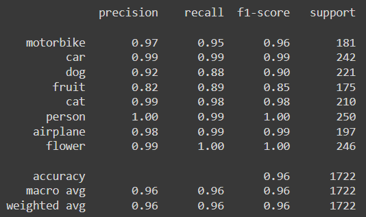
val_labels = np.argmax(val_labels, axis=1)

# show classification report 

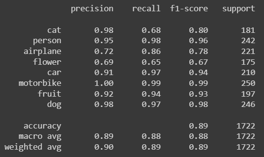
from sklearn.metrics import classification_report 

print(classification_report(val_labels, predicted_labels, target_names=classes))

# function to plot confusion matrix

import itertools

def plot_confusion_matrix(actual, predicted):

    cm = confusion_matrix(actual, predicted)
    cm = cm.astype('float') / cm.sum(axis=1)[:, np.newaxis]

    plt.figure(figsize=(7,7))
    cmap=plt.cm.Blues
    plt.imshow(cm, interpolation='nearest', cmap=cmap)
    plt.title('Confusion matrix', fontsize=25)
  
    tick_marks = np.arange(len(classes))
    plt.xticks(tick_marks, classes, rotation=90, fontsize=15)
    plt.yticks(tick_marks, classes, fontsize=15)

    thresh = cm.max() / 2.
    for i, j in itertools.product(range(cm.shape[0]), range(cm.shape[1])):
        plt.text(j, i, format(cm[i, j], '.2f'),
        horizontalalignment="center",
        color="white" if cm[i, j] > thresh else "black", fontsize = 14)

    plt.ylabel('True label', fontsize=20)
    plt.xlabel('Predicted label', fontsize=20)
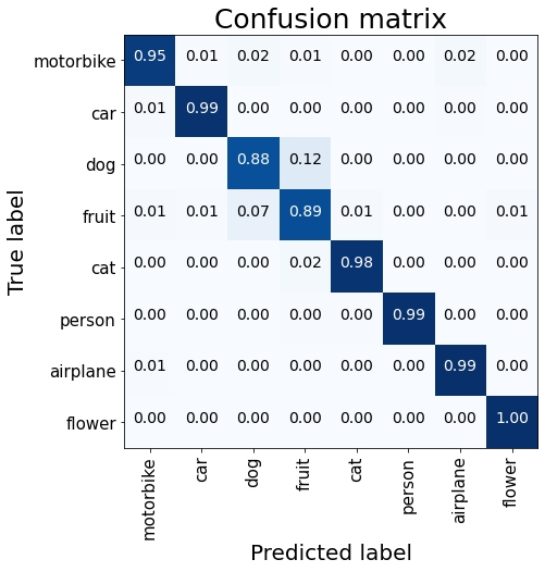
    plt.show()

# plot confusion matrix
plot_confusion_matrix(val_labels, predicted_labels)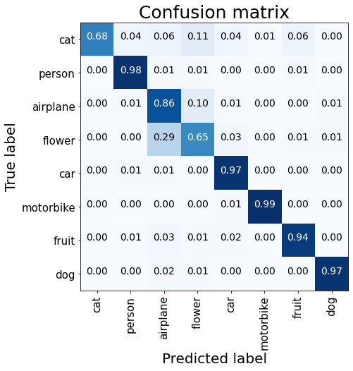

From the model evaluation, we notice that the custom model could not properly identify the images of cats and flowers. It also gives sub-optimal precision for identifying aeroplanes.

Next, we would try out a different model-building technique, by using weights learned by networks pre-trained on the Imagenet dataset to boost our model's performance in the classes with lower accuracy scores.

2. Using a pre-trained VGG16 model.

for our second model ,we would be using the VGG16 model pre-trained on the Imagenet dataset to train a model for our use case. This allows us to inherit the weights learned from training on a similar dataset to boost our model's performance.

Initializing and fine-tuning the VGG16 model.

# Import the VGG16 pretrained model 
from tensorflow.keras.applications import VGG16 

# initialize the model vgg16 = VGG16(input_shape=(224,224,3), weights='imagenet', include_top=False) 

# Freeze all but the last 3 layers for layer in vgg16.layers[:-3]: layer.trainable = False 

# build model 
input = vgg16.layers[-1].output # input is the last output from vgg16 

x = Dropout(0.25)(input) 
x = Flatten()(x) 
output = Dense(8, activation='softmax')(x) 

# create the model 
vgg16_model = Model(vgg16.input, output, name='VGG16_Model')

We initialize the pre-trained model and freeze all but the last three layers so we can utilize the weights of the models and learn new information in the last 3 layers that are specific to our use case. We also add a dropout layer to regularize the model from overfitting on our dataset before adding our final output layer.

We can then train our VGG16 fine-tuned model using similar training configurations to our custom model.

# compile the model 
vgg16_model.compile(optimizer= SGD(learning_rate=1e-3), loss= 'categorical_crossentropy', metrics= ['accuracy']) 

# reinitialize callbacks 
checkpoint = ModelCheckpoint('VggModel.weights.hdf5', monitor='val_loss', verbose=1,save_best_only=True, mode= 'min') 

callbacks= [reduceLR, early_stopping,checkpoint] 

# Train model 
vgg16_model.fit(train_gen, steps_per_epoch= TRAIN_STEPS, validation_data=val_gen, validation_steps=VAL_STEPS, epochs= epochs, callbacks= callbacks)

After training, we can evaluate the model's performance using similar scripts from the last model evaluation.

# Evaluate the model 
vgg16_model.evaluate(val_gen)

# get the model predictions 
predicted_labels = np.argmax(vgg16_model.predict(val_gen), axis=1) 

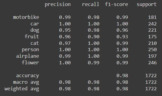
# show classification report 
print(classification_report(val_labels, predicted_labels, target_names=classes)) 

# plot confusion matrix 
plot_confusion_matrix(val_labels, predicted_labels)

Using a pre-trained VGG16 model produced better performance, especially for the classes with lower scores.

Finally, before ensembling, we would use another pre-trained model with much lesser parameters than the VGG16. The aim is to utilize different architectures so we can benefit from their varying properties to improve the quality of our final model. We would be using the Mobilenet model pre-trained on the same Imagenet dataset.

3. Using a pre-trained Mobilenet model.

For our final model, we would be finetuning the mobilenet model

# initializing the mobilenet model
mobilenet = MobileNet(input_shape=(224,224,3), weights='imagenet', include_top=False)

# freezing all but the last 5 layers
for layer in mobilenet.layers[:-5]:
  layer.trainable = False

# add few mor layers
x = mobilenet.layers[-1].output
x = Dropout(0.5)(x)
x = Flatten()(x) 
x = Dense(32, activation='relu')(x)
x = Dropout(0.5)(x)
x = Dense(16, activation='relu')(x)
output = Dense(8, activation='softmax')(x)

# Create the model
mobilenet_model = Model(mobilenet.input, output, name= "Mobilenet_Model")

For training the model, we maintain some of the previous configurations from our previous training.

# compile the model 
mobilenet_model.compile(optimizer= SGD(learning_rate=1e-3), loss= 'categorical_crossentropy', metrics= ['accuracy']) 

# reinitialize callbacks 
checkpoint = ModelCheckpoint('MobilenetModel.weights.hdf5', monitor='val_loss', verbose=1,save_best_only=True, mode= 'min') 

callbacks= [reduceLR, early_stopping,checkpoint] 

# model training 
mobilenet_model.fit(train_gen, steps_per_epoch= TRAIN_STEPS, validation_data=val_gen, validation_steps=VAL_STEPS, epochs=epochs, callbacks= callbacks)

After training our fine-tuned Mobilenet model, we can then evaluate its performance.

# Evaluate the model 
mobilenet_model.evaluate(val_gen) 

# get the model's predictions 
predicted_labels = np.argmax(mobilenet_model.predict(val_gen), axis=1) 

# show the classification report 
print(classification_report(val_labels, predicted_labels, target_names=classes)) 

# plot the confusion matrix 
plot_confusion_matrix(val_labels, predicted_labels)

The fine-tuned Mobilenet model performs better than the previous models and notably improves the identification of dogs and flowers.

While it would be fine to use the trained Mobilenet model or any of our models as our final choice, combining the structure and weights of the three models might prove better in developing a single, more generalizable model in production.

Ensembling The Models

To ensemble the models, we would be using three different ensembling methods as earlier stated: Concatenation, Average and Weighted Average.

The methods have their pros and cons which are often considered to determine the choice for a particular use case.

Concatenation Ensemble

This involves merging the parameters of multiple models into a single model. This is made possible in Tensorflow by the concatenation layer which receives inputs of tensors of the same shape (except for the concatenation axis) and merges them into one. This layer can therefore be used to merge all the information learnt by the different models side by side on a single axis into a single model. See here for more information about the Tensorflow concatenation layer.

To merge our models, we would simply input our models into the concatenation layer.

# concatenate the models

# import concatenate layer
from tensorflow.keras.layers import Concatenate

# get list of models
models = [custom_model, vgg16_model, mobilenet_model] 

input = Input(shape=(224, 224, 3), name='input') # input layer

# get output for each model input
outputs = [model(input) for model in models]

# contenate the ouputs
x = Concatenate()(outputs) 

# add further layers
x = Dropout(0.5)(x) 
output = Dense(8, activation='softmax', name='output')(x) # output layer

# create concatenated model
conc_model = Model(input, output, name= 'Concatenated_Model')

After concatenation, we added further layers as deemed appropriate for our task. In this example, I have added a dropout layer and a final output layer with the appropriate output dimensions of our use case.

Let's check the structure of our concatenated model.

# show model structure 
from tensorflow.keras.utils import plot_model 
plot_model(conc_model)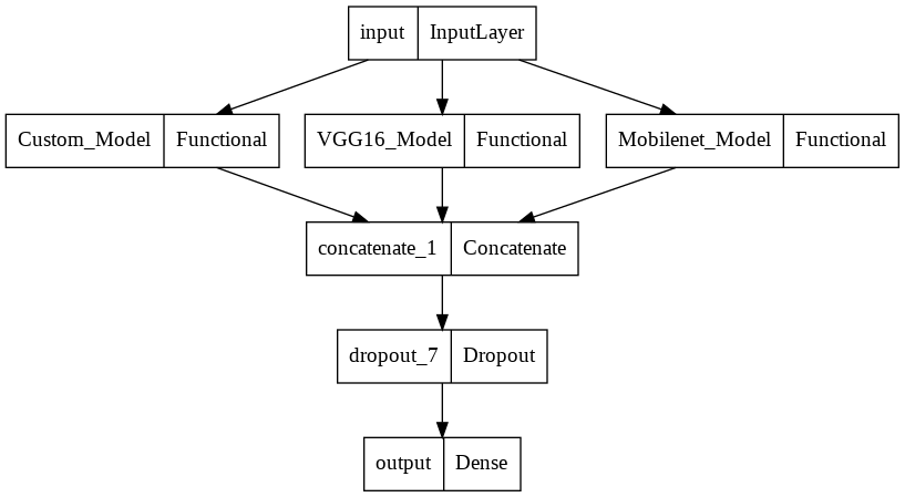

We can see how the three different functional models we've built are merged into one with further dropout and output layers.

This could prove useful for certain cases as we are utilizing all the information gained by the different models. The problem with this method is that the dimension of our final model is a concatenation of the dimensions of all the ensemble members which could lead to a dimensionality explosion, the inclusion of irrelevant information and consequently, overfitting.

Average Ensemble

Rather than risk exploding the model's dimension and overfitting for simpler tasks by concatenating multiple models, we could simply make our final model the average of all our models. This way, we are able to maintain a reasonable average dimension for our final model while utilizing the information of all our models.

This time we will use the Tensorflow Average layer which receives inputs and outputs their average. Therefore our final model is an average of the parameters of our input models. See here for more information about the average layer.

To ensemble our model by average,  we simply combine our models at the average layer.

# average ensemble model 

# import Average layer
from tensorflow.keras.layers import Average 

input = Input(shape=(224, 224, 3), name='input')  # input layer

# get output for each input model
outputs = [model(input) for model in models] 

# take average of the outputs
x = Average()(outputs) 

x = Dense(16, activation='relu')(x) 
x = Dropout(0.3)(x) 
output = Dense(8, activation='softmax', name='output')(x) # output layer

# create average ensembled model
avg_model = Model(input, output)

As previously seen,  further layers can be added to the network as deemed fit. We can also see the structure of the Average ensembled model.

# show model structure 
plot_model(avg_model)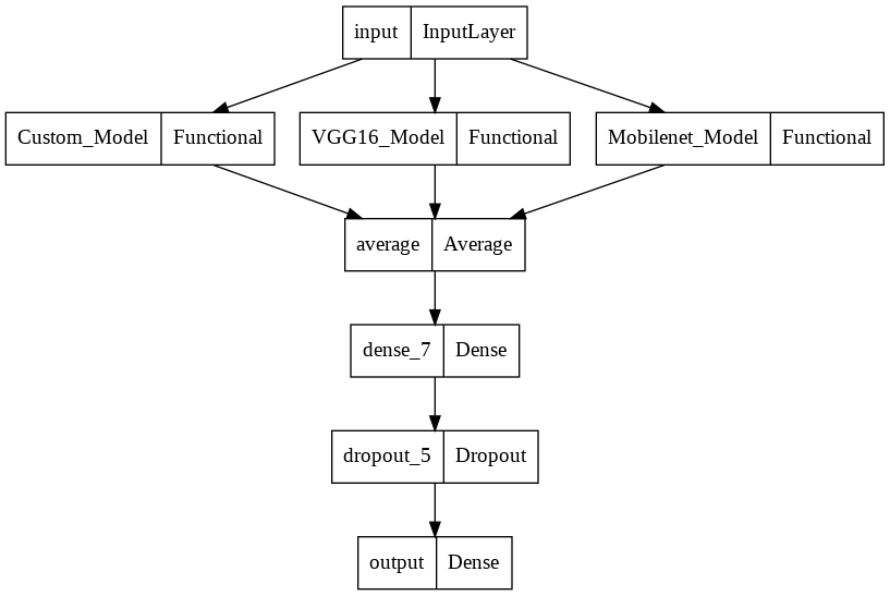

This approach to ensembling is particularly useful because by taking an average, the lower performance for certain classes is boosted by models with higher performance for such classes, thereby improving the model's overall performance and generalization.

The downside to this approach is that by taking the average, certain information from the models would not be included in the final model. Another is that because we are taking a simple average, the superiority and relevance of certain models are lost. As in our use case, the superiority in performance of the Mobilenet Model over other models is lost.

This could be resolved by taking a weighted average of the models when ensembling, such that it reflects the importance of each model to the final decision.

Weighted Average Ensemble

In weighted average ensembling, the outputs of the models are multiplied by an assigned weight and an average is taken to get a final model.  By assigning weights to the models when ensembling this way, we preserve their importance and contribution to the final decision.

While TensorFlow does not have a built-in layer for weighted average ensembling, we could utilize attributes of the built-in Layer class to implement a custom weighted average ensemble layer. For a weighted average ensemble, it is necessary that the weights sum up to one, we can ensure this by applying a softmax function on the weights before ensembling. You can see more about creating custom layers in TensorFlow here.

Implementing a custom weighted average layer

First, we define a custom function to set our weights.

# function for setting weights

import numpy as np

def weight_init(shape =(1,1,3), weights=[1,2,3], dtype=tf.float32):
    return tf.constant(np.array(weights).reshape(shape), dtype=dtype)

Here we have set a weight of 1,2 and 3 for our models respectively. We can then build our custom weighted average layer.

# implement custom weighted average layer

import tensorflow as tf
from tensorflow.keras.layers import Layer, Concatenate

class WeightedAverage(Layer):

    def __init__(self):
        super(WeightedAverage, self).__init__()
        
    def build(self, input_shape):
        
        self.W = self.add_weight(
                    shape=(1,1,len(input_shape)),
                    initializer=weighted_init,
                    dtype=tf.float32,
                    trainable=True)
    def call(self, inputs):
    
        inputs = [tf.expand_dims(i, -1) for i in inputs]
        inputs = Concatenate(axis=-1)(inputs) 
        weights = tf.nn.softmax(self.W, axis=-1)

        return tf.reduce_mean(weights*inputs, axis=-1)
    

To build our custom weighted average layer, we inherited attributes of the built-in Layer class and added weights using our weights initializing function. We apply a softmax to our initialized weights so that they sum up to one before multiplying it with the models.  Finally, we get the mean reduction of the weighted inputs to get our final model.

We can then ensemble our model using the custom weighted average layer.

input = Input(shape=(224, 224, 3), name='input')  # input layer

# get output for each input model
outputs = [model(input) for model in models] 

# get weighted average of outputs
x = WeightedAverage()(outputs)

output = Dense(8, activation='softmax')(x) # output layer

weighted_avg_model = Model(input, output, name= 'Weighted_AVerage_Model')

Let's check the structure of our weighted average model.

# plot model
plot_model(weighted_avg_model)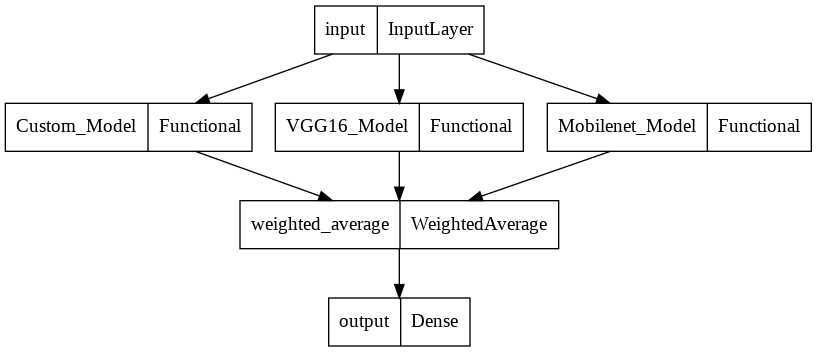

As in the previous methods, our models are ensembled, but this time, as a weighted average of the three models. The output dimension of the ensembled model is also compatible with the required output dimension for our task without adding any further layers.

Also, rather than manually set our weights using a custom weight initializing function, we could also utilize Tensorflow built-in weight initializers to initialize weights that are optimized during training. See here for the available built-in weight initializers in Tensorflow.

Summary

Model ensembling provides methods of combining multiple models to boost the performance and generalization of machine learning models. Neural networks can be combined using Tensorflow by concatenation, average or custom weighted average methods. All the information from the ensemble members is preserved using the concatenation technique at the risk of dimension explosion. Using the average method maintains a reasonable dimension for our model but loses certain information and does not account for the importance of each contributing model. This can be resolved by using a custom weighted average with weights that are optimized during the training process. There is also the possibility of extending  Neural Network ensembling using other operations.