Audio Classification with Deep Learning

Want to run the code in this article? Follow this link to run this code in a Gradient Notebook, or create your own by using this repo as the Notebook's "Workspace URL" in the advanced options of the Notebook creation page.

Visuals and sounds are two of the more common things that humans perceive. Both of these senses seem quite trivial for most people to analyze and develop an intuitive understanding of. Similar to how problems related to natural processing (NLP) are straightforward enough for humans to deal with, the same cannot be said for machines, as they have struggled to achieve desirable results in the past. However, with the introduction and rise of deep learning models and architectures over the last decade, we have been able to compute complex computations and projects with a much higher success rate.

In our previous blogs, we have discussed the multiple different types of problems and solutions to computer vision and natural language processing in detail. In this article and in upcoming future works, we will learn more about how deep learning models can be utilized to solve audio classification tasks as well as be used for music generation. The audio classification project is what we will focus on for this article and seek to achieve good results with simple architectures. The code and project can be computed on the Gradient Platform of Paperspace to reproduce and recreate the code snippets in this article.

Introduction:

Audio classification is the process of analyzing and identifying any type of audio, sound, noise, musical notes, or any other similar type of data to classify them accordingly. The audio data that is available to us can occur in numerous forms, such as sound from acoustic devices, musical chords from instruments, human speech, or even naturally occurring sounds like the chirping of birds in the environment. Modern deep learning techniques allow us to achieve state-of-the-art results for tasks and projects related to audio signal processing.

In this article, our primary objective is to gain a definitive understanding of the audio classification project while learning about the essential basic concepts of signal processing and some of the best techniques utilized to achieve the desired outcomes. Before diving into the contents of this article, I would first recommend getting more familiar with deep learning frameworks and other essential basic concepts. You can check out more information on the TensorFlow (link) and Keras (link) libraries, which we will utilize for the construction of this project. Let us understand some of the basic concepts of audio classification.

Exploring the Basic Concepts of Audio Classification:

In this section of the article, we will try to understand some of the useful terms that are essential for understanding audio classification with deep learning. We will explore some of the basic terminologies that we may come across during our work on audio processing projects. Let us get started by analyzing some of these key concepts in brief.

Waveform:

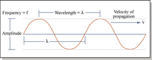
Before we analyze the waveform and its numerous parameters, let us understand what sound is. Sound is the vibrations produced by an object when the air particles in the surrounding oscillate. The respective changes in the air pressure create these sound waves. Sound is a mechanical wave where energy is transferred from one source to another. A waveform is a schematic representation that helps us to analyze the displacement of sound waves over time, along with some of the other essential parameters that are required for a specific task.

On the other hand, the frequency in a waveform is the representation of the number of times that a waveform repeats itself within a one-second time period. The peak of the waveform at the top is called a crest, whereas the bottom point is called the trough. Amplitude is the distance from the center line to the top of a trough or the bottom of a crest. With a brief understanding and grasp of these basic concepts, we can proceed to visit some of the other essential topics required for audio classification.

Spectrograms:

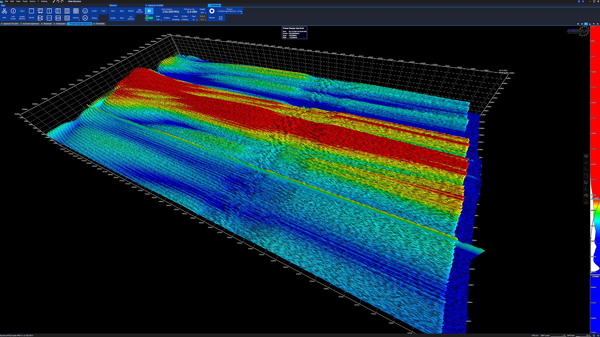
Spectrograms are the visual representations of the spectrum of frequencies in an audio signal. Other technical terms for spectrograms are sonographs, voiceprints, or voicegrams. These spectrograms are used extensively in the field of signal processing, music generation, audio classification, linguistic analysis, speech detection, and so much more. We will also use spectrograms in this article for the task of audio classification. For further information on this topic, I would recommend checking out the following link.

Audio Signal Processing:

Audio signal processing is the field that deals with audio signals, sound waves, and other manipulations of audio frequencies. When talking specifically about deep learning for audio signal processing, we have numerous applications that we can work on in this large field.

In this article, we will cover the topic of audio classification in greater detail. Some of the other major applications include speech recognition, audio denoising, sound information retrieval, music generation, and so much more. The combination of deep learning to solve audio signal processing tasks has numerous possibilities and is worth exploring. Let us proceed to understand the audio classification project in the next section before proceeding further toward its implementation from scratch.

Understanding the Audio Classification Project:

Audio classification is one of the best basic introductory projects to get started with audio deep learning. The objective is to understand the waveforms that are available in the raw format and convert the existing data into a form that is usable by the developers. By converting a raw waveform of the audio data into the form of spectrograms, we can pass it through deep learning models to interpret and analyze the data. In audio classification, we normally perform a binary classification in which we determine if the input signal is our desired audio or not.

In this project, our objective is to retrieve an incoming sound made by a bird. The incoming noise signal is converted into a waveform that we can utilize for further processing and analysis with the help of the TensorFlow deep learning framework. Once the waveform is obtained successfully, we can proceed to convert this waveform into a spectrogram, which is a visual representation of the available waveform. Since these spectrograms are visual images, we can make use of convolutional neural networks to analyze them accordingly by creating a deep learning model to compute a binary classification result.

Implementation of the Audio Classification and Recognition project with Deep Learning:

As discussed previously, the objective of our project is to read the incoming sounds from a forest and interpret whether the received data belongs to a specific bird (capuchin bird) or is some other noise that we are not really interested in acknowledging. For the construction of this entire project, we will make use of the TensorFlow and Keras deep learning frameworks.

You can check out the following article to learn more about TensorFlow and the Keras article here. The other additional installation that is required for this project is the TensorFlow-io library, which will grant us access to file systems and file formats that are not available in TensorFlow's built-in support. The following pip command provided below can be used to install the library in your working environment.

pip install tensorflow-io[tensorflow]

Importing the essential libraries:

In the next step, we will import all the essential libraries that are required for the construction of the following project. For this project, we will use a Sequential type model that will allow us to construct a simple convolutional neural network to analyze the spectrograms produced and achieve a desirable result. Since the architecture of the model developed is quite simple, we do not really need to make use of the functional model API or the custom modeling functionality.

We will make use of the convolutional layers for the architecture as well as some Dense and flatten layers. As discussed earlier, we will also utilize the TensorFlow input output library for handling a larger number of file systems and formats such as the .wav format and the .mp3 formats. The Operating System library import will help us to access all the required files in their respective formats

import tensorflow as tf 
from tensorflow.keras.models import Sequential
from tensorflow.keras.layers import Conv2D, Dense, Flatten
import tensorflow_io as tfio
from matplotlib import pyplot as plt
import os

Loading the dataset:

The dataset for this project is obtainable through the Kaggle Challenge for Signal Processing - Z by HP Unlocked Challenge 3, which you can download from this link.

Once the dataset is downloaded and extracted, we can notice three directories in the data folder. The three directories are namely the forest recordings containing a three-minute clip of the sounds produced in the forest, three seconds clips of Capuchin bird recordings, and three-second recording clips of sounds not produced by the Capuchin birds. In the next code snippet, we will define variables to set these paths accordingly.

CAPUCHIN_FILE = os.path.join('data', 'Parsed_Capuchinbird_Clips', 'XC3776-3.wav')
NOT_CAPUCHIN_FILE = os.path.join('data', 'Parsed_Not_Capuchinbird_Clips', 'afternoon-birds-song-in-forest-0.wav')

In the next step, we will define the data loading function that will be useful for creating the required waveforms in the desired format for further computation. The function defined in the code snippet below will allow us to read the data and convert it into a mono (or single) channel for easier analysis. We will also vary the frequency signals allowing us to modify the overall amplitude to achieve smaller data samples for the overall analysis.

def load_wav_16k_mono(filename):
    # Load encoded wav file
    file_contents = tf.io.read_file(filename)
    # Decode wav (tensors by channels) 
    wav, sample_rate = tf.audio.decode_wav(file_contents, desired_channels=1)
    # Removes trailing axis
    wav = tf.squeeze(wav, axis=-1)
    sample_rate = tf.cast(sample_rate, dtype=tf.int64)
    # Goes from 44100Hz to 16000hz - amplitude of the audio signal
    wav = tfio.audio.resample(wav, rate_in=sample_rate, rate_out=16000)
    return wav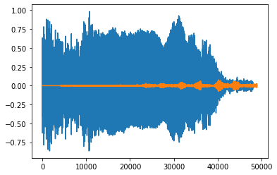

The above image represents the waveform Plot of Capuchin and Non-Capuchin signals.

Preparing the dataset:

In this section of the article, we will define the positive and negative paths for the Capuchin bird clips. The positive paths variables store the path to the directory containing the clip recordings of the Capuchin birds, while the negative paths are stored in another variable. We will link the files in these directories to the .wav formats and add their respective labels. The labels are in terms of binary classification and are labeled as 0 or 1. The positive labels are assigned with a value of one, which means the clip contains the audio signal of a Capuchin bird. The negative labels with zeros indicate that the audio signals are random noises that do not contain clip recordings of Capuchin birds.

# Defining the positive and negative paths
POS = os.path.join('data', 'Parsed_Capuchinbird_Clips/*.wav')
NEG = os.path.join('data', 'Parsed_Not_Capuchinbird_Clips/*.wav')

# Creating the Datasets
pos = tf.data.Dataset.list_files(POS)
neg = tf.data.Dataset.list_files(NEG)

# Adding labels
positives = tf.data.Dataset.zip((pos, tf.data.Dataset.from_tensor_slices(tf.ones(len(pos)))))
negatives = tf.data.Dataset.zip((neg, tf.data.Dataset.from_tensor_slices(tf.zeros(len(neg)))))
data = positives.concatenate(negatives)

We can also analyze the average wavelength of the Capuchin bird, as shown in the code snippet below, by loading in the positive samples directory and loading our previously created data loading function.

# Analyzing the average wavelength of a Capuchin bird
lengths = []
for file in os.listdir(os.path.join('data', 'Parsed_Capuchinbird_Clips')):
    tensor_wave = load_wav_16k_mono(os.path.join('data', 'Parsed_Capuchinbird_Clips', file))
    lengths.append(len(tensor_wave))

The minimum, mean, and maximum wave length cycles, respectively, are provided below.

<tf.Tensor: shape=(), dtype=int32, numpy=32000>

<tf.Tensor: shape=(), dtype=int32, numpy=54156>

<tf.Tensor: shape=(), dtype=int32, numpy=80000>

Converting Data to Spectrograms:

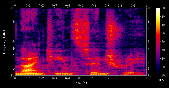
In the next step, we will create the function to complete the pre-processing steps required for audio analysis. We will convert the previously acquired waveforms into the form of spectrograms. These visualized audio signals in the form of spectrograms will be used by our deep learning model in the upcoming steps to analyze and interpret the results accordingly. In the below code block, we acquire all the waveforms and compute the Short-time Fourier Transform of signals with the TensorFlow library to acquire a visual representation, as shown in the image provided below.

def preprocess(file_path, label): 
    for i in os.listdir(file_path):
        i = file_path.decode() + "/" + i.decode()
        wav = load_wav_16k_mono(i)
        wav = wav[:48000]
        zero_padding = tf.zeros([48000] - tf.shape(wav), dtype=tf.float32)
        wav = tf.concat([zero_padding, wav],0)
        spectrogram = tf.signal.stft(wav, frame_length=320, frame_step=32)
        spectrogram = tf.abs(spectrogram)

        spectrogram = tf.expand_dims(spectrogram, axis=2)
        return spectrogram, label

 
filepath, label = positives.shuffle(buffer_size=10000).as_numpy_iterator().next()

spectrogram, label = preprocess(filepath, label)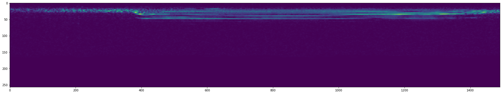

Building the deep learning Model:

Before we start constructing the deep learning model, let us create the data pipeline by loading the data. We will load in the spectrogram data elements that are obtained from the pre-processing step function. We can cache and shuffle this data by using the TensorFlow in-built functionalities, as well as create a batch size of sixteen to load the data elements accordingly. Before we proceed to construct the deep learning model, we can create partitions for the training and testing samples, as shown in the below code snippet.

# Creating a Tensorflow Data Pipeline
data = data.map(preprocess)
data = data.cache()
data = data.shuffle(buffer_size=1000)
data = data.batch(16)
data = data.prefetch(8)

# Split into Training and Testing Partitions
train = data.take(36)
test = data.skip(36).take(15)

In the next step, we will build a Sequential type model. We can develop the architecture to solve the task with a functional API or custom model archetype. We can then proceed to add the convolutional layers with the respective shape of the sample label to build two blocks of convolutional layers with sixteen filters and a kernel size of (3, 3). The ReLU activation function is utilized in the construction of the convolutional layers. We can then proceed to flatten the acquired output from the convolutional layers to make it suitable for further processing. Finally, we can add the fully connected layers with the Sigmoid activation function with one output node to receive the binary classification output. The code snippet and the summary of the model constructed are shown below.

model = Sequential()
model.add(Conv2D(16, (3,3), activation='relu', input_shape=(1491, 257,1)))
model.add(Conv2D(16, (3,3), activation='relu'))
model.add(Flatten())
# model.add(Dense(128, activation='relu'))
model.add(Dense(1, activation='sigmoid'))

model.summary()

Model: "sequential"
_________________________________________________________________
 Layer (type)                Output Shape              Param #   
=================================================================
 conv2d (Conv2D)             (None, 1489, 255, 16)     160       
                                                                 
 conv2d_1 (Conv2D)           (None, 1487, 253, 16)     2320      
                                                                 
 flatten (Flatten)           (None, 6019376)           0         
                                                                 
 dense (Dense)               (None, 1)                 6019377   
                                                                 
=================================================================
Total params: 6,021,857
Trainable params: 6,021,857
Non-trainable params: 0
_________________________________________________________________

Once we have completed the building of the model architecture, we can proceed to compile and train the model accordingly. For the compilation of the model, we can use the Adam optimizer, the binary cross-entropy loss function for the binary classification, and define some additional recall and precision metrics for the model analysis. We can train the data that we previously built with the validation test data and fit the model for a few epochs. The code snippet and result obtained after this step is shown below.

# Compiling and fitting the model
model.compile('Adam', loss='BinaryCrossentropy', metrics=[tf.keras.metrics.Recall(),tf.keras.metrics.Precision()])

model.fit(train, epochs=4, validation_data=test)

Epoch 1/4
36/36 [==============================] - 204s 6s/step - loss: 1.6965 - recall: 0.8367 - precision: 0.8483 - val_loss: 0.0860 - val_recall: 0.9254 - val_precision: 0.9688
Epoch 2/4
36/36 [==============================] - 200s 6s/step - loss: 0.0494 - recall: 0.9477 - precision: 0.9932 - val_loss: 0.0365 - val_recall: 1.0000 - val_precision: 0.9846
Epoch 3/4
36/36 [==============================] - 201s 6s/step - loss: 0.0314 - recall: 0.9933 - precision: 0.9801 - val_loss: 0.0228 - val_recall: 0.9821 - val_precision: 1.0000
Epoch 4/4
36/36 [==============================] - 201s 6s/step - loss: 0.0126 - recall: 0.9870 - precision: 1.0000 - val_loss: 0.0054 - val_recall: 1.0000 - val_precision: 0.9861

Once we have constructed the model and trained it successfully, we can analyze and validate the results. The metrics obtained in the results show good progress. And hence, we can deem the constructed model suitable for making relatively successful predictions on the bird calls to identify the noise frequency of the Capuchin birds. In the next section, we will look into the steps for this procedure.

Making the required Predictions:

In the final step of this project, we will analyze how to make the appropriate predictions on all the existing files in forest recordings. Before that step, let us look at how to make a prediction on a single batch, as shown in the code snippet below.

# Prediction for a single batch
X_test, y_test = test.as_numpy_iterator().next()
yhat = model.predict(X_test)

# converting logits to classes
yhat = [1 if prediction > 0.5 else 0 for prediction in yhat]

Now that we have looked at how to make predictions for a single batch, it is essential to note how we can make predictions on the files present in the forest recordings directory. Each of the clips in the forest recordings is about three minutes long. Since our predictions consist of a three-second clip for detecting the Capuchin bird calls, we can segment these longer clips into windowed spectrums. We can divide the three-minute-long clips (180 seconds) into sixty smaller fragments to perform the analysis. We will detect the total Capuchin bird calls in this section, where each clip has a score of zero or one.

Once we determine the calls for every windowed spectrum, we can compute the total number of counts in the entire clip by adding all the individual values. The total counts tell us the number of times a Capuchin bird sound was heard throughout the audio clip. In the code snippet below, we will build our first function similar to the one discussed in the previous section, where we read the forest recording clips, which are in the form of mp3 files as opposed to .wav format. The function below takes the mp3 format input and converts them into tensors. We then compute the average of the multi-channel input to convert it into a mono channel and obtain the desired frequency signal.

def load_mp3_16k_mono(filename):
    """ Load an audio file, convert it to a float tensor, resample to 16 kHz single-channel audio. """
    res = tfio.audio.AudioIOTensor(filename)
    # Convert to tensor and combine channels 
    tensor = res.to_tensor()
    tensor = tf.math.reduce_sum(tensor, axis=1) / 2 
    # Extract sample rate and cast
    sample_rate = res.rate
    sample_rate = tf.cast(sample_rate, dtype=tf.int64)
    # Resample to 16 kHz
    wav = tfio.audio.resample(tensor, rate_in=sample_rate, rate_out=16000)
    return wav
    
mp3 = os.path.join('data', 'Forest Recordings', 'recording_00.mp3')

wav = load_mp3_16k_mono(mp3)

audio_slices = tf.keras.utils.timeseries_dataset_from_array(wav, wav, sequence_length=48000, sequence_stride=48000, batch_size=1)

samples, index = audio_slices.as_numpy_iterator().next()

In the next code snippet, we will construct a function that will help us to segregate the individual fragments into windowed spectrograms for further computation. We will map the data accordingly and create the appropriate slices for making the required predictions, as shown below.

# Build Function to Convert Clips into Windowed Spectrograms
def preprocess_mp3(sample, index):
    sample = sample[0]
    zero_padding = tf.zeros([48000] - tf.shape(sample), dtype=tf.float32)
    wav = tf.concat([zero_padding, sample],0)
    spectrogram = tf.signal.stft(wav, frame_length=320, frame_step=32)
    spectrogram = tf.abs(spectrogram)
    spectrogram = tf.expand_dims(spectrogram, axis=2)
    return spectrogram
    
audio_slices = tf.keras.utils.timeseries_dataset_from_array(wav, wav, sequence_length=16000, sequence_stride=16000, batch_size=1)
audio_slices = audio_slices.map(preprocess_mp3)
audio_slices = audio_slices.batch(64)

yhat = model.predict(audio_slices)
yhat = [1 if prediction > 0.5 else 0 for prediction in yhat]

In the final code snippet of this article, we will run the following process for all the files in the forest recordings and obtain a total computed result. The results will contain clips of zeros and ones where the total of the ones is outputted to compute the overall score of the clips. We can find out the total number of Capuchin bird calls in the audio recordings as required in the following project with the code provided below.

results = {}
class_preds = {}

for file in os.listdir(os.path.join('data', 'Forest Recordings')):
    FILEPATH = os.path.join('data','Forest Recordings', file)
    
    wav = load_mp3_16k_mono(FILEPATH)
    audio_slices = tf.keras.utils.timeseries_dataset_from_array(wav, wav, sequence_length=48000, sequence_stride=48000, batch_size=1)
    audio_slices = audio_slices.map(preprocess_mp3)
    audio_slices = audio_slices.batch(64)
    
    yhat = model.predict(audio_slices)
    
    results[file] = yhat
    
for file, logits in results.items():
    class_preds[file] = [1 if prediction > 0.99 else 0 for prediction in logits]
class_preds

The two primary references for this project are the notebook from Kaggle and the following GitHub link. Most of the code is taken from the following references, and I would highly recommend checking them out. The code for this blogpost is also hosted on Gradient AI. Create a Notebook with this URL as the Workspace URL to load this code as an .ipynb directly into a Notebook.

There are several additional improvements that can be made to this project to achieve better results. The complexity of the network can be increased as well as other innovative methods can be utilized to obtain more precision in the analysis of the Capuchin bird patterns. We will also look at some other projects related to audio signal processing in future articles.

Conclusion:

Audio signal processing with deep learning has garnered high traction due to its high rate of success in interpreting and accomplishing a wide array of complex projects. Most of the complicated signaling projects, such as acoustic music detection, audio classification, environmental sound classification, and so much more, can be achieved through deep learning techniques. With further improvements and advancements in these fields, we can expect greater feats of accomplishments.

In this article, we were introduced to audio classification with deep learning. We explored and analyzed some of the basic and essential components required to thoroughly understand the concept of audio classification. We then had a brief summary of the particular project of this blog before proceeding to the implementation section of the task. We made use of the TensorFlow framework for conversion of waveforms, used the spectrograms for analysis, and constructed a simple convolutional neural capable of binary classification of audio data. There are several improvements that could be added to the following project to achieve better results.

In the upcoming articles, we will look at more intriguing projects related to audio signal processing with deep learning. We will also analyze some music generation projects and continue our work with Generative adversarial networks and neural networks from scratch. Until then, have fun exploring and building new projects!