How to Build a Variational Autoencoder in Keras

This tutorial gives an introduction to the variational autoencoder (VAE) neural network, how it differs from typical autoencoders, and its benefits. We'll then build a VAE in Keras that can encode and decode images.

The outline of this tutorial is as follows:

• Introduction to Variational Autoencoders
• Building the Encoder
• Building the Decoder
• Building the VAE
• Training the VAE
• A Look at the Code
• Testing the model

You can follow along with the full code on the ML Showcase.

Introduction to Variational Autoencoders

An autoencoder is a type of convolutional neural network (CNN) that converts a high-dimensional input into a low-dimensional one (i.e. a latent vector), and later reconstructs the original input with the highest quality possible. It consists of two connected CNNs. The first is an encoder network that accepts the original data as input, and returns a vector. This vector is then fed to the second CNN, the decoder that reconstructs the original data. For more information about the architecture you can check out the tutorial Image Compression Using Autoencoders in Keras, also on the Paperspace blog.

One problem with autoencoders is that they encode each sample of the data independently of other samples, even if they are from the same class. But if two samples are of the same class, there should be some relationship between the encoded versions. Formalizing this discussion, we can say that this problem is due to the fact that the autoencoder does not follow a pre-defined distribution to encode the data.

In other words, let's say we have two samples from the same class, S1 and S2. Each sample will be encoded independently, so that S1 is encoded into E1 ad S2 is encoded into E2. When E1 and E2 are decoded there is no guarantee that the reconstructed samples will be similar, because each sample is treated independently.

This leaves things ambiguous. After the data is encoded, each sample is encoded into a vector. Assuming the vector length is 2, then what would be the range of values for each element in the vector? Is it from -1 to 1? Or 0 to 5? Or 100 to 200? The answer is unknown because there is nothing forcing the vector to be within a certain range. You might train the encoder network and find that the range is -10 to 20, for example. Another time it might change to be -15 to 12. You'll have to explore the encoded data to deduce the range of values for the vector.

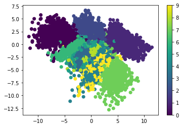
The next figure shows the latent vector of MNIST samples compressed using an autoencoder (have a look at this tutorial for more details). The range is nearly from -2.5 to 15.0. Sure, it might change when the network is trained again, especially when the parameters change.

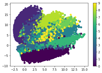
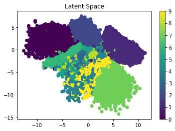
The variational autoencoder solves this problem by creating a defined distribution representing the data. VAEs try to force the distribution to be as close as possible to the standard normal distribution, which is centered around 0. So, when you select a random sample out of the distribution to be decoded, you at least know its values are around 0. The next figure shows how the encoded samples using the VAE are distributed. As you can see, the samples are centered around 0.

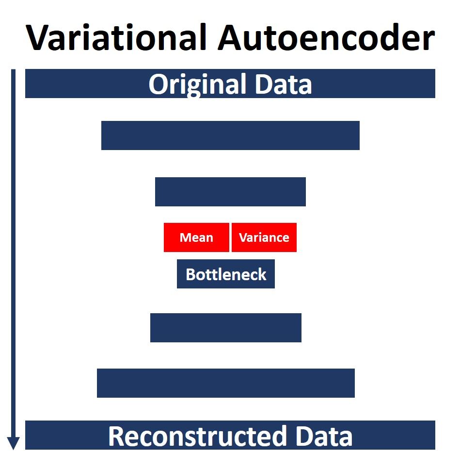
Because a normal distribution is characterized based on the mean and the variance, the variational autoencoder calculates both for each sample and ensures they follow a standard normal distribution (so that the samples are centered around 0). There are two layers used to calculate the mean and variance for each sample. So, on a high level you can imagine the architecture as what is shown in the next figure.

(For more information about VAEs, I recommend this book: Generative Deep Learning: Teaching Machines to Paint, Write, Compose, and Play by David Foster.)

Now that we have an overview of the VAE, let's use Keras to build the encoder.

Building the Encoder

In this tutorial we'll focus on how to build the VAE in Keras, so we'll stick to the basic MNIST dataset in order to avoid getting distracted from the code. Of course, you can easily swap this out for your own data of interest.

The images in this dataset are binary, with a width and height of 28 pixels. As a result, the single image size is 28x28x1. Note that there is a single channel in the image. The next line creates two variables to hold the size and number of channels in the image.

img_size = 28
num_channels = 1

We'll use these variables to create the input layer of the encoder, according to the next line.

x = tensorflow.keras.layers.Input(shape=(img_size, img_size, num_channels), name="encoder_input")

Following the input layer are a number of combinations of the following three layers:

1. 2D Convolution
2. Batch Normalization
3. Leaky ReLU

Here is the code for creating the first combination of these layers.

encoder_conv_layer1 = tensorflow.keras.layers.Conv2D(filters=1, kernel_size=(3, 3), padding="same", strides=1, name="encoder_conv_1")
encoder_norm_layer1 = tensorflow.keras.layers.BatchNormalization(name="encoder_norm_1")(encoder_conv_layer1)
encoder_activ_layer1 = tensorflow.keras.layers.LeakyReLU(name="encoder_leakyrelu_1")(encoder_norm_layer1)

The next code block creates the other combinations of conv-norm-relu layers.

encoder_conv_layer2 = tensorflow.keras.layers.Conv2D(filters=32, kernel_size=(3,3), padding="same", strides=1, name="encoder_conv_2")(encoder_activ_layer1)
encoder_norm_layer2 = tensorflow.keras.layers.BatchNormalization(name="encoder_norm_2")(encoder_conv_layer2)
encoder_activ_layer2 = tensorflow.keras.layers.LeakyReLU(name="encoder_activ_layer_2")(encoder_norm_layer2)

encoder_conv_layer3 = tensorflow.keras.layers.Conv2D(filters=64, kernel_size=(3,3), padding="same", strides=2, name="encoder_conv_3")(encoder_activ_layer2)
encoder_norm_layer3 = tensorflow.keras.layers.BatchNormalization(name="encoder_norm_3")(encoder_conv_layer3)
encoder_activ_layer3 = tensorflow.keras.layers.LeakyReLU(name="encoder_activ_layer_3")(encoder_norm_layer3)

encoder_conv_layer4 = tensorflow.keras.layers.Conv2D(filters=64, kernel_size=(3,3), padding="same", strides=2, name="encoder_conv_4")(encoder_activ_layer3)
encoder_norm_layer4 = tensorflow.keras.layers.BatchNormalization(name="encoder_norm_4")(encoder_conv_layer4)
encoder_activ_layer4 = tensorflow.keras.layers.LeakyReLU(name="encoder_activ_layer_4")(encoder_norm_layer4)

encoder_conv_layer5 = tensorflow.keras.layers.Conv2D(filters=64, kernel_size=(3,3), padding="same", strides=1, name="encoder_conv_5")(encoder_activ_layer4)
encoder_norm_layer5 = tensorflow.keras.layers.BatchNormalization(name="encoder_norm_5")(encoder_conv_layer5)
encoder_activ_layer5 = tensorflow.keras.layers.LeakyReLU(name="encoder_activ_layer_5")(encoder_norm_layer5)

The size of the output from the last layer in the previous architecture is (7, 7, 64). So, the image size is reduced from 28x28 to just 7x7, and the number of channels is now 64. Because a VAE converts multi-dimensional data into a vector, the output must be converted into a 1D vector using a dense layer (as shown below). The purpose of the shape_before_flatten variable is to hold the shape of the result before being flattened, in order to decode the result successfully.

shape_before_flatten = tensorflow.keras.backend.int_shape(encoder_activ_layer5)[1:]
encoder_flatten = tensorflow.keras.layers.Flatten()(encoder_activ_layer5)

In a regular autoencoder, converting the data into a vector marks the end of the encoder. This is not the case for a VAE. The reason is that a VAE creates a standard normal distribution to represent the data. For this purpose, the parameters of the distribution (mean and variance) must be taken into account. The following code creates two layers for these two parameters.

latent_space_dim = 2

encoder_mu = tensorflow.keras.layers.Dense(units=latent_space_dim, name="encoder_mu")(encoder_flatten)
encoder_log_variance = tensorflow.keras.layers.Dense(units=latent_space_dim, name="encoder_log_variance")(encoder_flatten)

The units parameter in the Dense class constructor is set equal to latent_space_dim, which is a variable set to 2, representing the length of the latent vector. If you want to create a latent vector of any length, just specify the proper value for the latent_space_dim variable.

Using these two layers, encoder_mu and encoder_log_variance, the normal distribution is randomly sampled to return the output of the encoder. The next line creates a custom Lambda layer for this purpose. For more information about the Lambda layer in Keras, check out the tutorial Working With The Lambda Layer in Keras.

encoder_output = tensorflow.keras.layers.Lambda(sampling, name="encoder_output")([encoder_mu, encoder_log_variance])

The Lambda layer calls a function named sampling(), which is implemented as follows.

def sampling(mu_log_variance):
    mu, log_variance = mu_log_variance
    epsilon = tensorflow.keras.backend.random_normal(shape=tensorflow.keras.backend.shape(mu), mean=0.0, stddev=1.0)
    random_sample = mu + tensorflow.keras.backend.exp(log_variance/2) * epsilon
    return random_sample

Now the encoder architecture from the input layer to the output layer is complete. The final remaining step is to create a model that associates the input layer to the output layer of the encoder, according to the next line.

encoder = tensorflow.keras.models.Model(x, encoder_output, name="encoder_model")

Here is the complete code for building the encoder of the VAE.

# Encoder
x = tensorflow.keras.layers.Input(shape=(img_size, img_size, num_channels), name="encoder_input")

encoder_conv_layer1 = tensorflow.keras.layers.Conv2D(filters=1, kernel_size=(3, 3), padding="same", strides=1, name="encoder_conv_1")(x)
encoder_norm_layer1 = tensorflow.keras.layers.BatchNormalization(name="encoder_norm_1")(encoder_conv_layer1)
encoder_activ_layer1 = tensorflow.keras.layers.LeakyReLU(name="encoder_leakyrelu_1")(encoder_norm_layer1)

encoder_conv_layer2 = tensorflow.keras.layers.Conv2D(filters=32, kernel_size=(3,3), padding="same", strides=1, name="encoder_conv_2")(encoder_activ_layer1)
encoder_norm_layer2 = tensorflow.keras.layers.BatchNormalization(name="encoder_norm_2")(encoder_conv_layer2)
encoder_activ_layer2 = tensorflow.keras.layers.LeakyReLU(name="encoder_activ_layer_2")(encoder_norm_layer2)

encoder_conv_layer3 = tensorflow.keras.layers.Conv2D(filters=64, kernel_size=(3,3), padding="same", strides=2, name="encoder_conv_3")(encoder_activ_layer2)
encoder_norm_layer3 = tensorflow.keras.layers.BatchNormalization(name="encoder_norm_3")(encoder_conv_layer3)
encoder_activ_layer3 = tensorflow.keras.layers.LeakyReLU(name="encoder_activ_layer_3")(encoder_norm_layer3)

encoder_conv_layer4 = tensorflow.keras.layers.Conv2D(filters=64, kernel_size=(3,3), padding="same", strides=2, name="encoder_conv_4")(encoder_activ_layer3)
encoder_norm_layer4 = tensorflow.keras.layers.BatchNormalization(name="encoder_norm_4")(encoder_conv_layer4)
encoder_activ_layer4 = tensorflow.keras.layers.LeakyReLU(name="encoder_activ_layer_4")(encoder_norm_layer4)

encoder_conv_layer5 = tensorflow.keras.layers.Conv2D(filters=64, kernel_size=(3,3), padding="same", strides=1, name="encoder_conv_5")(encoder_activ_layer4)
encoder_norm_layer5 = tensorflow.keras.layers.BatchNormalization(name="encoder_norm_5")(encoder_conv_layer5)
encoder_activ_layer5 = tensorflow.keras.layers.LeakyReLU(name="encoder_activ_layer_5")(encoder_norm_layer5)

shape_before_flatten = tensorflow.keras.backend.int_shape(encoder_activ_layer5)[1:]
encoder_flatten = tensorflow.keras.layers.Flatten()(encoder_activ_layer5)

encoder_mu = tensorflow.keras.layers.Dense(units=latent_space_dim, name="encoder_mu")(encoder_flatten)
encoder_log_variance = tensorflow.keras.layers.Dense(units=latent_space_dim, name="encoder_log_variance")(encoder_flatten)

encoder_mu_log_variance_model = tensorflow.keras.models.Model(x, (encoder_mu, encoder_log_variance), name="encoder_mu_log_variance_model")

def sampling(mu_log_variance):
    mu, log_variance = mu_log_variance
    epsilon = tensorflow.keras.backend.random_normal(shape=tensorflow.keras.backend.shape(mu), mean=0.0, stddev=1.0)
    random_sample = mu + tensorflow.keras.backend.exp(log_variance/2) * epsilon
    return random_sample

encoder_output = tensorflow.keras.layers.Lambda(sampling, name="encoder_output")([encoder_mu, encoder_log_variance])

encoder = tensorflow.keras.models.Model(x, encoder_output, name="encoder_model")

To summarize the architecture of the encoder, the encoder.summary() command is issued. Below is the result. There are a total of 105,680 trainable parameters. The size of the output is (None, 2), which means it returns a vector of length 2 for each input. Note that the shape of the layer exactly before the flatten layer is (7, 7, 64), which is the value saved in the shape_before_flatten variable.

Note that you are free to change the values of parameters in the layers, and add or remove layers to customize the model to your application.

_________________________________________________________________________________________
Layer (type)                    Output Shape         Param #  Connected to                     
=========================================================================================
encoder_input (InputLayer)      [(None, 28, 28, 1)]  0                                   
_________________________________________________________________________________________
encoder_conv_1 (Conv2D)         (None, 28, 28, 1)    10       encoder_input[0][0]     
_________________________________________________________________________________________
encoder_norm_1 (BatchNormalizat (None, 28, 28, 1)    4        encoder_conv_1[0][0]     
_________________________________________________________________________________________
encoder_leakyrelu_1 (LeakyReLU) (None, 28, 28, 1)    0        encoder_norm_1[0][0]       
_________________________________________________________________________________________
encoder_conv_2 (Conv2D)         (None, 28, 28, 32)   320      encoder_leakyrelu_1[0][0]   
_________________________________________________________________________________________
encoder_norm_2 (BatchNormalizat (None, 28, 28, 32)   128      encoder_conv_2[0][0]       
_________________________________________________________________________________________
encoder_activ_layer_2 (LeakyReL (None, 28, 28, 32)   0        encoder_norm_2[0][0]       
_________________________________________________________________________________________
encoder_conv_3 (Conv2D)         (None, 14, 14, 64)   18496    encoder_activ_layer_2[0][0]
_________________________________________________________________________________________
encoder_norm_3 (BatchNormalizat (None, 14, 14, 64)   256      encoder_conv_3[0][0]     
_________________________________________________________________________________________
encoder_activ_layer_3 (LeakyReL (None, 14, 14, 64)   0        encoder_norm_3[0][0]     
_________________________________________________________________________________________
encoder_conv_4 (Conv2D)         (None, 7, 7, 64)     36928    encoder_activ_layer_3[0][0]      
_________________________________________________________________________________________
encoder_norm_4 (BatchNormalizat (None, 7, 7, 64)     256      encoder_conv_4[0][0]     
_________________________________________________________________________________________
encoder_activ_layer_4 (LeakyReL (None, 7, 7, 64)     0        encoder_norm_4[0][0]     
_________________________________________________________________________________________
encoder_conv_5 (Conv2D)         (None, 7, 7, 64)     36928    encoder_activ_layer_4[0][0]      
_________________________________________________________________________________________
encoder_norm_5 (BatchNormalizat (None, 7, 7, 64)     256      encoder_conv_5[0][0]       
_________________________________________________________________________________________
encoder_activ_layer_5 (LeakyReL (None, 7, 7, 64)     0        encoder_norm_5[0][0]     
_________________________________________________________________________________________
flatten (Flatten)               (None, 3136)         0        encoder_activ_layer_5[0][0] 
_________________________________________________________________________________________
encoder_mu (Dense)              (None, 2)            6274     flatten[0][0]           
_________________________________________________________________________________________
encoder_log_variance (Dense)    (None, 2)            6274     flatten[0][0]               
_________________________________________________________________________________________
encoder_output (Lambda)         (None, 2)            0        encoder_mu[0][0]         
                                                              encoder_log_variance[0][0] 
=========================================================================================
Total params: 106,130
Trainable params: 105,680
Non-trainable params: 450
_________________________________________________________________________________________

Now that we've built the encoder network, let's build our decoder.

Building the Decoder

In the previous section, the encoder accepted an input of shape (28, 28) and returned a vector of length 2. In this section, the decoder should do the reverse: accept an input vector of length 2, and return a result of shape (28, 28).

The first step is to create a layer which holds the input, according to the line below. Note that the shape for the input is set equal to latent_space_dim, which was previously assigned a value of 2. This means the input for the decoder will be a vector of length 2.

decoder_input = tensorflow.keras.layers.Input(shape=(latent_space_dim), name="decoder_input")

The next step is to create a dense layer that expands the length of the vector from 2 to the value specified into the shape_before_flatten variable, which is (7, 7, 64). numpy.prod() is used to multiply the three values and return just a single value. Now, the shape of the dense layer is (None, 3136).

decoder_dense_layer1 = tensorflow.keras.layers.Dense(units=numpy.prod(shape_before_flatten), name="decoder_dense_1")(decoder_input)

The next step is to reshape the result from a vector to a matrix using the Reshape layer.

decoder_reshape = tensorflow.keras.layers.Reshape(target_shape=shape_before_flatten)(decoder_dense_layer1)

After that, we can add a number of layers that expand the shape until reaching the desired shape of the original input, (28, 28).

decoder_conv_tran_layer1 = tensorflow.keras.layers.Conv2DTranspose(filters=64, kernel_size=(3, 3), padding="same", strides=1, name="decoder_conv_tran_1")(decoder_reshape)
decoder_norm_layer1 = tensorflow.keras.layers.BatchNormalization(name="decoder_norm_1")(decoder_conv_tran_layer1)
decoder_activ_layer1 = tensorflow.keras.layers.LeakyReLU(name="decoder_leakyrelu_1")(decoder_norm_layer1)

decoder_conv_tran_layer2 = tensorflow.keras.layers.Conv2DTranspose(filters=64, kernel_size=(3, 3), padding="same", strides=2, name="decoder_conv_tran_2")(decoder_activ_layer1)
decoder_norm_layer2 = tensorflow.keras.layers.BatchNormalization(name="decoder_norm_2")(decoder_conv_tran_layer2)
decoder_activ_layer2 = tensorflow.keras.layers.LeakyReLU(name="decoder_leakyrelu_2")(decoder_norm_layer2)

decoder_conv_tran_layer3 = tensorflow.keras.layers.Conv2DTranspose(filters=64, kernel_size=(3, 3), padding="same", strides=2, name="decoder_conv_tran_3")(decoder_activ_layer2)
decoder_norm_layer3 = tensorflow.keras.layers.BatchNormalization(name="decoder_norm_3")(decoder_conv_tran_layer3)
decoder_activ_layer3 = tensorflow.keras.layers.LeakyReLU(name="decoder_leakyrelu_3")(decoder_norm_layer3)

decoder_conv_tran_layer4 = tensorflow.keras.layers.Conv2DTranspose(filters=1, kernel_size=(3, 3), padding="same", strides=1, name="decoder_conv_tran_4")(decoder_activ_layer3)
decoder_output = tensorflow.keras.layers.LeakyReLU(name="decoder_output")(decoder_conv_tran_layer4 )

Now the architecture of the decoder is complete. The remaining step is to create a model that links the input and output of the decoder.

decoder = tensorflow.keras.models.Model(decoder_input, decoder_output, name="decoder_model")

Here is the summary of the decoder model.

_________________________________________________________________
Layer (type)                 Output Shape              Param #   
=================================================================
decoder_input (InputLayer)   [(None, 2)]               0         
_________________________________________________________________
decoder_dense_1 (Dense)      (None, 3136)              9408      
_________________________________________________________________
reshape (Reshape)            (None, 7, 7, 64)          0         
_________________________________________________________________
decoder_conv_tran_1 (Conv2DT (None, 7, 7, 64)          36928     
_________________________________________________________________
decoder_norm_1 (BatchNormali (None, 7, 7, 64)          256       
_________________________________________________________________
decoder_leakyrelu_1 (LeakyRe (None, 7, 7, 64)          0         
_________________________________________________________________
decoder_conv_tran_2 (Conv2DT (None, 14, 14, 64)        36928     
_________________________________________________________________
decoder_norm_2 (BatchNormali (None, 14, 14, 64)        256       
_________________________________________________________________
decoder_leakyrelu_2 (LeakyRe (None, 14, 14, 64)        0         
_________________________________________________________________
decoder_conv_tran_3 (Conv2DT (None, 28, 28, 64)        36928     
_________________________________________________________________
decoder_norm_3 (BatchNormali (None, 28, 28, 64)        256       
_________________________________________________________________
decoder_leakyrelu_3 (LeakyRe (None, 28, 28, 64)        0         
_________________________________________________________________
decoder_conv_tran_4 (Conv2DT (None, 28, 28, 1)         577       
_________________________________________________________________
decoder_output (LeakyReLU)   (None, 28, 28, 1)         0         
=================================================================
Total params: 121,537
Trainable params: 121,153
Non-trainable params: 384
_________________________________________________________________

After building the architectures of both the encoder and the decoder, the remaining step is to create the full VAE.

Building the VAE

In the previous two sections, two separate models for the encoder and decoder were created. In this section we will build a third model that combines the two.

One question to answer is: why build a model for the VAE if we already have the encoder and decoder? The reason is that we need to train both the encoder and the decoder at the same time, and we cannot do so when the models are separated from each other.

After completing the architectures of the encoder and the decoder, building the architecture of the VAE is so simple. All we need to do is create an input layer representing the input to the VAE (which is identical to that of the encoder).

vae_input = tensorflow.keras.layers.Input(shape=(img_size, img_size, num_channels), name="VAE_input")

The VAE input layer is then connected to the encoder to encode the input and return the latent vector.

vae_encoder_output = encoder(vae_input)

The output of the encoder is then connected to the decoder to reconstruct the input.

vae_decoder_output = decoder(vae_encoder_output)

Finally, the model of the VAE that links the encoder to the decoder is created.

vae = tensorflow.keras.models.Model(vae_input, vae_decoder_output, name="VAE")

Here is the summary of the VAE model.

_________________________________________________________________
Layer (type)                 Output Shape              Param #   
=================================================================
VAE_input (InputLayer)       [(None, 28, 28, 1)]       0         
_________________________________________________________________
encoder_model (Model)        (None, 2)                 106130    
_________________________________________________________________
decoder_model (Model)        (None, 28, 28, 1)         121537    
=================================================================
Total params: 227,667
Trainable params: 226,833
Non-trainable params: 834
_________________________________________________________________

Before starting training, the VAE model is compiled as follows.

vae.compile(optimizer=tensorflow.keras.optimizers.Adam(lr=0.0005), loss=loss_func(encoder_mu, encoder_log_variance))

The implementation of the loss function is given below.

def loss_func(encoder_mu, encoder_log_variance):
    def vae_reconstruction_loss(y_true, y_predict):
        reconstruction_loss_factor = 1000
        reconstruction_loss = tensorflow.keras.backend.mean(tensorflow.keras.backend.square(y_true-y_predict), axis=[1, 2, 3])
        return reconstruction_loss_factor * reconstruction_loss

    def vae_kl_loss(encoder_mu, encoder_log_variance):
        kl_loss = -0.5 * tensorflow.keras.backend.sum(1.0 + encoder_log_variance - tensorflow.keras.backend.square(encoder_mu) - tensorflow.keras.backend.exp(encoder_log_variance), axis=1)
        return kl_loss

    def vae_kl_loss_metric(y_true, y_predict):
        kl_loss = -0.5 * tensorflow.keras.backend.sum(1.0 + encoder_log_variance - tensorflow.keras.backend.square(encoder_mu) - tensorflow.keras.backend.exp(encoder_log_variance), axis=1)
        return kl_loss

    def vae_loss(y_true, y_predict):
        reconstruction_loss = vae_reconstruction_loss(y_true, y_predict)
        kl_loss = vae_kl_loss(y_true, y_predict)

        loss = reconstruction_loss + kl_loss
        return loss

    return vae_loss

Now we're ready to train our model.

Training the VAE

Before training, the data must be loaded. Fortunately, the MNIST dataset can be loaded using Keras according to this command tensorflow.keras.datasets.mnist.load_data(). Here is how the train and test data is loaded.

(x_train, y_train), (x_test, y_test) = tensorflow.keras.datasets.mnist.load_data() 
x_train = x_train.astype("float32") / 255.0 x_test = x_test.astype("float32") / 255.0

The shape of each image in the dataset is just (28, 28), and the model expects the shape to be (28, 28, 1). For this purpose, the shape of the train and test data is changed as follows:

x_train = numpy.reshape(x_train, newshape=(x_train.shape[0], x_train.shape[1], x_train.shape[2], 1)) 
x_test = numpy.reshape(x_test, newshape=(x_test.shape[0], x_train.shape[1], x_train.shape[2], 1))

Finally, the VAE training can begin. You can freely change the values assigned to the epochs and batch_size parameters.

vae.fit(x_train, x_train, epochs=20, batch_size=32, shuffle=True, validation_data=(x_test, x_test))

After model training completes, we can save the three models (encoder, decoder, and VAE) for later use.

encoder.save("VAE_encoder.h5") 
decoder.save("VAE_decoder.h5") 
vae.save("VAE.h5")

The next figure shows the latent space for the samples after being encoded using the VAE encoder. The samples are now centered around 0, which means the VAE is able to represent the encoded samples using a normal distribution.

Complete Code

Run the complete code for building and training the VAE for free on the ML Showcase.

Testing the VAE

For testing the VAE, we can start by loading the encoder and decoder models according to the next two lines.

encoder = tensorflow.keras.models.load_model("VAE_encoder.h5") 
decoder = tensorflow.keras.models.load_model("VAE_decoder.h5")

We also have to make sure the data is loaded.

(x_train, y_train), (x_test, y_test) = tensorflow.keras.datasets.mnist.load_data() 

x_test = x_test.astype("float32") / 255.0  

x_test = numpy.reshape(x_test, newshape=(x_test.shape[0], x_train.shape[1], x_train.shape[2], 1))

Now, we are ready to encode and decode the test data.

encoded_data = encoder.predict(x_test)
decoded_data = decoder.predict(encoded_data)

Here is a summary of some images reconstructed using the VAE.

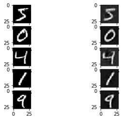
Summary

This tutorial introduced the variational autoencoder, a convolutional neural network used for converting data from a high-dimensional space into a low-dimensional one, and then reconstructing it.

The advantage of the VAE compared to the vanilla autoencoder is that it models the distribution of the data as a standard normal distribution centered around 0.

Using Keras, we implemented a VAE to compress the images of the MNIST dataset. The models for the encoder, decoder, and the VAE are saved to be loaded later for testing purposes. For any comments or questions, feel free to reach out in the comments.