Generative Adversarial Networks are one of the most useful concepts to learn in modern deep learning. They have a wide range of applications, including one where the user can have more control of the type of data that will be generated. While simple generative networks are quite capable of handling different types of problems and achieving the necessary solutions, there are numerous variations of these generative networks to accomplish more specific tasks in order to achieve the best possible results. One such similar Generative network architecture that we will explore in this article is the concept of Conditional Generative Adversarial Networks (CGANs).

In our previous blogs, we have discussed numerous types of Generative Adversarial Networks (GANs) such as DCGAN, WGAN, SRGAN, and many more. In this article, we will focus on conditional GANs to allow us more control over the type of data that is generated.

We will first look at a brief introduction of this concept, and proceed to understand an intuitive understanding of conditional GANs. We will construct a project with the CGAN architecture, and finally, look at some applications of these generative networks. I would recommend using the Paperspace Gradient platform for running this program and other similar codes for achieving high-end results.

Introduction:

When running a simple generative adversarial network (GAN), the trained generator network might generate a variety of images that it was developed to create. There is not a way to get complete control on the type of data that we aim to generate with these simple networks, which might sometimes be required if you train the data on a larger dataset but need to generate a specific type of data (or image) that you are looking for. One of the variations of GANs that make this a possibility where you can specify the exact type of data or image you want to generate is the conditional Generative Adversarial Networks (CGANs).

Before proceeding into further sections, I would highly recommend getting familiar with Generative Adversarial Networks from the following article. I have covered most of the elementary concepts of GANs in the mentioned blog. Since CGAN is a variation of the simple GAN architecture, it is extremely beneficial to have some knowledge and understanding of GAN architectures. The classes or labels are the essential addition to both the discriminator and generator network that will enable us to train the model to train conditionally. A minor variation in the simple GAN architecture results in the new CGAN architecture that allows us to generate the outputs for exactly the classes or labels that we desire. Let us explore these concepts further in the upcoming sections.

Understanding Conditional GANs:

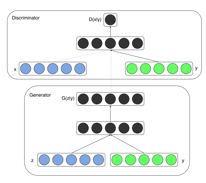
In our previous works, we have explored GANs where we have no control over the type of output that is being produced. Unlike most generative network architectures, CGANs are not completely unsupervised in their training methods. These CGAN network architectures require some kind of class labels or labeled data to perform the desired action. Let us understand the difference between a simple GAN architecture and a CGAN architecture with some mathematical formulas. Firstly, let us explore the mathematical expression for the GAN structure, as shown below.

The formula expression represents a min-max type of algorithm, where we are trying to reduce (or minimize) the variation in the discriminator and generator networks while both the generator and discriminator models are being trained simultaneously. We are aiming to achieve a generator that generates a high-quality output that can bypass an efficient discriminator network. However, we do not have control over the type of output generated in such an architecture. Let us now look at the CGAN mathematical expression that allows us to achieve the desired results.

With a minor modification to our previous formula of the simple GAN architecture, we have now added a y-label to both the discriminator and the generator network. By converting the previous probabilities into conditional probabilities with the addition of the 'y'-labels, we can ensure that the training generator and discriminator networks are now trained only for the respective label. Hence, we can send a particular input label and receive the desired output from the generative network once the training procedure is complete.

Both the generator and discriminator networks will have these labels assigned to them during the training process. Hence, both these networks of the CGAN architecture are trained conditionally such that the generator generates only outputs similar to the expected label output, while the discriminator model ensures to check if the generated output is real or fake alongside checking if the image matches the particular label. Now that we have developed a brief intuitive understanding of Conditional GANs, we can proceed to construct the CGAN architecture for solving the MNIST project.

Building the CGAN architecture:

In this section of the article, we will focus on building the Conditional GAN architecture with both the generator and discriminator structures. For the MNIST task, we will assign each of the digits from 0-9 as the respective labels for the conditional GANs. Once the labels are assigned, the conditional GAN will produce the appropriate images for the assigned digits. This generation is different from the images generated by a simple GAN network where random images with no fixed conditions would be generated. We will make use of the TensorFlow and Keras deep learning frameworks for building the CGAN architectural network.

Before proceeding with the rest of this section, I would recommend checking out the following article to learn more about TensorFlow and the Keras article from here.

Let us now get started with the library imports.

Importing the required libraries:

from tensorflow.keras.layers import UpSampling2D, Reshape, Activation, Conv2D, BatchNormalization, LeakyReLU, Input, Flatten, multiply
from tensorflow.keras.layers import Dense, Embedding
from tensorflow.keras.layers import Dropout, Concatenate
from tensorflow.keras.models import Sequential, Model
from tensorflow.keras.datasets import mnist

import matplotlib.pyplot as plt
import numpy as np
import warnings 

warnings.filterwarnings('ignore')
from tensorflow.python.client import device_lib
print(device_lib.list_local_devices())

Firstly, let us import all the essential libraries and modules that we will require for constructing the conditional GAN (CGAN) architecture. Most of the layers will be utilized for the construction of the CGAN model network. If you have learned about my previous GAN articles, these networks should be quite familiar. Most of the CGAN architecture will follow a basic GAN structure with the addition of labels to train the model. For converting the labels into a vector format, we will make use of the embedding layers. All the layers will be loaded from the TensorFlow and Keras deep learning frameworks. Below is the code snippet for all the necessary imports.

Assigning the essential requirements:

(X_train,y_train),(X_test,y_test) = mnist.load_data()

img_width, img_height =28,28
img_channel = 1
img_shape = (img_width, img_height, img_channel)
num_classes = 10
z_dim = 100

X_train.shape

Output:

(60000, 28, 28)

Since we will be using the MNIST dataset for this project, let us load the data into the training and testing samples. We will declare the required parameters such as the image height, image width, and the number of channels. Each of the images in the MNIST dataset are of the size 28 x 28 and are grayscale image with one channel. We have a total of ten classes, which will act as the labels for our CGAN model to learn. A default z-dimensional space of 100 is defined. The code snippet for the following is shown below.

Constructing the generator architecture:

def build_generator():
    model = Sequential()
    model.add(Dense(128*7*7, activation = 'relu', input_shape = (z_dim, )))
    model.add(Reshape((7,7,128)))
    model.add(UpSampling2D())
    model.add(Conv2D(128, kernel_size = 3, strides = 2, padding = 'same'))
    model.add(BatchNormalization())
    model.add(LeakyReLU(alpha = 0.02))
    model.add(UpSampling2D())
    model.add(Conv2D(64, kernel_size = 3, strides = 1, padding = 'same'))
    model.add(BatchNormalization())
    model.add(LeakyReLU(alpha = 0.02))
    model.add(UpSampling2D())
    model.add(Conv2D(1, kernel_size = 3 , strides = 1, padding='same'))
    model.add(Activation('tanh'))
    
    z = Input(shape= (z_dim,))
    label = Input(shape=(1,), dtype = 'int32')
    
    label_embedding = Embedding(num_classes, z_dim, input_length = 1)(label)
    label_embedding = Flatten()(label_embedding)
    joined = multiply([z, label_embedding])
    
    img = model(joined)
    return Model([z, label], img)

generator = build_generator()
generator.summary()

Output:

Model: "model"
__________________________________________________________________________________________________
Layer (type)                    Output Shape         Param #     Connected to                     
==================================================================================================
input_2 (InputLayer)            [(None, 1)]          0                                            
__________________________________________________________________________________________________
embedding (Embedding)           (None, 1, 100)       1000        input_2[0][0]                    
__________________________________________________________________________________________________
input_1 (InputLayer)            [(None, 100)]        0                                            
__________________________________________________________________________________________________
flatten (Flatten)               (None, 100)          0           embedding[0][0]                  
__________________________________________________________________________________________________
multiply (Multiply)             (None, 100)          0           input_1[0][0]                    
                                                                 flatten[0][0]                    
__________________________________________________________________________________________________
sequential (Sequential)         (None, 28, 28, 1)    856193      multiply[0][0]                   
==================================================================================================
Total params: 857,193
Trainable params: 856,809
Non-trainable params: 384
__________________________________________________________________________________________________

For building the generator and discriminator architecture, we will follow a similar scheme as the simple GAN architecture for the most part. We will firstly use a Sequential model archetype, and start building our model layers. We will use 128 matrices, each having a dimensionality of 7 x 7. We will then start using upsampling layers followed by convolutional layers. Batch normalization layers are also utilized, along with leaky ReLU layers having an alpha value of 0.02. We will continue using these building blocks until we obtain a final desired shape similar to the MNIST data. Finally, we will conclude with the tanh activation function, and this part of the function contains the image that will be generated by the generator with the randomly assigned noise.

In the second half of this function, we will add an embedding to create the vector mapping for the labels (or classes) that must be assigned accordingly. Each of the ten digits of the MNIST data must be treated as separate and unique labels, and the model must generate each of them accordingly. We can create these label embeddings and proceed to combine this information with our previous generator model. Once combined, we will return the overall model and store it in the generator variable.

Constructing the discriminator architecture:

def build_discriminator():
    model = Sequential()
    model.add(Conv2D(32, kernel_size = 3, strides = 2, input_shape = (28,28,2), padding = 'same'))
    model.add(BatchNormalization())
    model.add(LeakyReLU(alpha = 0.02))
    model.add(Conv2D(64, kernel_size = 3, strides = 2, padding = 'same'))
    model.add(BatchNormalization())
    model.add(LeakyReLU(alpha = 0.02))
    model.add(Conv2D(128, kernel_size = 3, strides = 2, padding = 'same'))
    model.add(BatchNormalization())
    model.add(LeakyReLU(alpha = 0.02))
    model.add(Dropout(0.25))
    model.add(Flatten())
    model.add(Dense(1, activation = 'sigmoid'))
    
    img = Input(shape= (img_shape))
    label = Input(shape= (1,), dtype = 'int32')
    
    label_embedding = Embedding(input_dim = num_classes, output_dim = np.prod(img_shape), input_length = 1)(label)
    label_embedding = Flatten()(label_embedding)
    label_embedding = Reshape(img_shape)(label_embedding)
    
    concat = Concatenate(axis = -1)([img, label_embedding])
    prediction = model(concat)
    return Model([img, label], prediction)

discriminator = build_discriminator()
discriminator.summary()

Output:

Model: "model_1"
__________________________________________________________________________________________________
Layer (type)                    Output Shape         Param #     Connected to                     
==================================================================================================
input_4 (InputLayer)            [(None, 1)]          0                                            
__________________________________________________________________________________________________
embedding_1 (Embedding)         (None, 1, 784)       7840        input_4[0][0]                    
__________________________________________________________________________________________________
flatten_2 (Flatten)             (None, 784)          0           embedding_1[0][0]                
__________________________________________________________________________________________________
input_3 (InputLayer)            [(None, 28, 28, 1)]  0                                            
__________________________________________________________________________________________________
reshape_1 (Reshape)             (None, 28, 28, 1)    0           flatten_2[0][0]                  
__________________________________________________________________________________________________
concatenate (Concatenate)       (None, 28, 28, 2)    0           input_3[0][0]                    
                                                                 reshape_1[0][0]                  
__________________________________________________________________________________________________
sequential_1 (Sequential)       (None, 1)            95905       concatenate[0][0]                
==================================================================================================
Total params: 103,745
Trainable params: 103,297
Non-trainable params: 448
__________________________________________________________________________________________________

Once we have finished constructing the generator network, we can proceed to build the discriminator architecture, which will function as the classifier. Firstly, let us construct the classifier network, which makes use of convolutional layers with strides of two that continuously resize the network. The batch normalization layers, along with the dropouts, are utilized to avoid the overfitting of the network. We also make use of the leaky ReLU activation function.

Finally, the Dense layer with the sigmoid activation function will classify the output as real or fake. A similar logic is used for the discriminator network. The labels are passed through the discriminator network as well as we need to ensure that these embeddings are available for both the generator and discriminator architectures.

Computing the results:

Now that we have finished constructing the generator and discriminator architecture for the CGAN model, we can finally begin the training procedure. We will divide this section into three different parts, namely compilation of the model, training and fitting the model, and finally, saving and displaying the results obtained after the training process is completed. Let us get started with each of these individual parts.

Compiling the model:

from tensorflow.keras.optimizers import Adam

discriminator.compile(loss = 'binary_crossentropy', optimizer = Adam(0.001, 0.5), metrics = ['accuracy'])

z = Input(shape=(z_dim,))
label = Input(shape= (1,))
img = generator([z,label])

# discriminator.trainable = False
prediction = discriminator([img, label])

cgan = Model([z, label], prediction)
cgan.compile(loss= 'binary_crossentropy', optimizer = Adam(0.001, 0.5))

For the compilation of the CGAN model, we will use the binary cross-entropy loss function, the Adam optimizer, a default learning rate of 0.001, and a beta1 value of 0.5. We will also set the discriminator to measure the accuracy at the end of each epoch. We will then assign the default parameters to be passed through the generator model, which are the z-dimensional space and the labels. We will then pass the generator and discriminator architectures for the conditional GAN network, and finally compile this model.

Defining the Generator and Discriminator training:

def train(epochs, batch_size, save_interval):
    (X_train, y_train), (_, _) = mnist.load_data()
    
    X_train = (X_train - 127.5) / 127.5
    X_train = np.expand_dims(X_train, axis=3)
    
    real = np.ones(shape=(batch_size, 1))
    fake = np.zeros(shape=(batch_size, 1))
    
    for iteration in range(epochs):
        
        idx = np.random.randint(0, X_train.shape[0], batch_size)
        imgs, labels = X_train[idx], y_train[idx]
        
        z = np.random.normal(0, 1, size=(batch_size, z_dim))
        gen_imgs = generator.predict([z, labels])
        
        d_loss_real = discriminator.train_on_batch([imgs, labels], real)
        d_loss_fake = discriminator.train_on_batch([gen_imgs, labels], fake)
        d_loss = 0.5 * np.add(d_loss_real, d_loss_fake)
        
        z = np.random.normal(0, 1, size=(batch_size, z_dim))
        labels = np.random.randint(0, num_classes, batch_size).reshape(-1, 1)
        
        g_loss = cgan.train_on_batch([z, labels], real)
        
        if iteration % save_interval == 0:
            print('{} [D loss: {}, accuracy: {:.2f}] [G loss: {}]'.format(iteration, d_loss[0], 100 * d_loss[1], g_loss))
            save_image(iteration)

Once the compilation of the model is done, we can proceed to define the generator and discriminator training mechanisms. The train function we define will take in the input values for the set number of epochs, the set batch size, and the inputted intervals in which the generated images are to be saved.

In the training method, we will pass random numbers and values to receive fake images. Both the discriminator and generator networks will be trained simultaneously, as shown in the below code above.

Saving and computing the training of the CGAN architecture:

Ensure that you create an images directory where all the images generated by the CGAN architecture can be stored. You can either do it manually in the Gradient GUI by creating a new folder in your working directory, in a terminal with mkdir images, or make use of the code snippet provided below.

import os

os.mkdir("images/")

Finally, let us define the last function that we will require for this project. We will create a function to save the images at the mentioned location and at the end of the specified interval. The matplotlib library is also utilized to plot the images and save them in the images directory. Below is the code block for performing the following action.

def save_image(epoch):
    r, c = 2,5
    z = np.random.normal(0,1,(r*c, z_dim))
    labels = np.arange(0,10).reshape(-1,1)
    gen_image = generator.predict([z,labels])
    gen_image = 0.5 * gen_image + 0.5
    
    fig, axes = plt.subplots(r,c, figsize = (10,10))
    count = 0
    for i in range(r):
        for j in range(c):
            axes[i,j].imshow(gen_image[count,:,:,0],cmap = 'gray')
            axes[i,j].axis('off')
            axes[i,j].set_title("Digit: %d" % labels[count])
            count+=1
    plt.savefig('images/cgan_%d.jpg' % epoch)
    plt.close()

We will train the model for about 5000 epochs with a batch size of 128 and save the images once after every 1000 epochs of training. Below is the code snippet to perform the following action for 5000 epochs, which saves 5 images to the directory.

# training the network
train(5000, 128, 1000)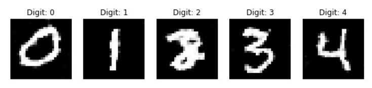

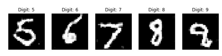
During the training process, you should be able to notice that at each of the 1000 intervals, we are saving an image, and the process of the CGAN model learning how to generate the specific images for the given label gradually increases. I would recommend checking out the following GitHub reference for this CGAN project from the mentioned links. Apart from the MNIST project, CGANs have numerous applications. We will cover these in detail in the upcoming section.

Applications of CGAN:

At first glance, it might be easy to wonder if CGANs find a lot of utility for most modern requirements. Now that we gained an intuitive and conceptual understanding of conditional GANs with the construction of this network, we can proceed to explore some of the most popular applications that you can utilize these conditional GANs. These generative architectures are extremely useful for some significant applications. Let us discuss a few of these important use cases that CGANs help to solve.

1. Image-to-image translation: In the application of image to image translation, we make use of an input image to map it to its respective output image. With the help of conditional GANs, we can specify the type of input image that we want as the particular condition and train the output images accordingly with respect to the input image. Given the particular input condition, one or more variations of the respective output can be generated. Another way to look at this application is the transformation of an image from an input domain into another domain. I would recommend checking out one of my previous articles to study a similar application using neural style transfer where we make use of content and style images to construct a generated image.
2. Text-to-image synthesis: The application of the text to image synthesis is similar to the one we worked on in this article. Given a text description, the generative network of CGAN can generate images for the particular description. In the example discussed in this blog, we are able to generate digits ranging from 0 - 9 given the respective label. There are also other examples where you can specify a condition, such as a particular animal in the text, and train the CGAN network to generate the specific image of the animal mentioned in the text.
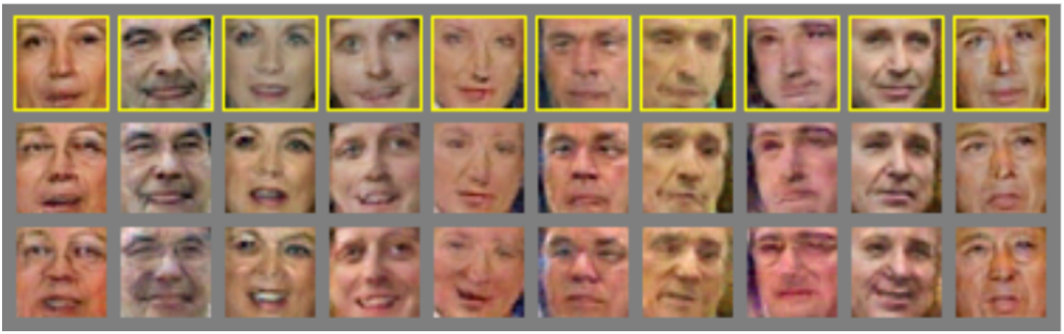
3. Convolutional face generation: In one of my previous articles, we have discussed the construction of a face generation project with Generative networks in great detail. With the help of conditional GANs, this application can have additional improvements in the facial generation patterns. We can train the model to make use of external factors to implement different modes of the same face. This can involve the generation of different kinds of emotions for a specific facial condition (please refer to the image displayed at the start of this section). For further information and understanding of convolutional face generation, I would recommend checking out the following research paper.
4. Video generation: Similar to the previously discussed application, we can make use of conditional GANs for video generation. We can specify a particular caption or video title and generate entire videos for the condition. A combination of all the generated faces can be combined together to create the movement of a moving face as well with a more structured approach. If you are interested in learning further details of such an application, I would recommend checking out the following research paper where the authors develop a Generative network for generating a video by encoding a caption.

There are a lot more practical applications for Conditional GANs that developers, researchers, and enthusiasts of AI can feel free to explore for their own specific use cases and practical applications. Since there is a huge variety of unique projects that we can develop with Conditional GANs, it is suggested that the viewers check out more such experiments and implement them accordingly.

Conclusion:

Generative Adversarial Networks provide some of the best ways for neural networks to learn and create content from the provided resources. Of the many different structures that we can construct with these generative networks, we can add a degree of supervision by adding labels. Given a particular label, when the generative network is able to generate the desired images for the respective class (or condition), we can create more replicable copies. Such conditional networks have a wide array of uses that developers can take advantage of to create unique projects.

In this article, we looked at another significant variation of generative networks in Conditional Generative Adversarial Networks (CGAN). With the help of conditional GANs, we saw how a user can specify a particular condition and generate the particular images for the specified label. We gained an intuitive understanding of conditional GANs, and learned how to construct their generative and discriminator architecture builds with labels. We also discussed some of the more popular applications of these conditional GANs and the numerous use cases in which they find their utility in.

In the upcoming articles, we will look into more variations of GANs and the high amount of utility they offer in Cycle GANs and Pix-To-Pix GANs. We will also look at some natural language processing applications with BERT and how to construct neural networks from scratch in future blogs. Until then, keep exploring and constructing new projects!