Are you working on a regression problem and looking for an efficient algorithm to solve your problem? If yes, you must explore gradient boosting regression (or GBR).
In this article we'll start with an introduction to gradient boosting for regression problems, what makes it so advantageous, and its different parameters. Then we'll implement the GBR model in Python, use it for prediction, and evaluate it.
Let's get started.

Introduction to Gradient Boosting Regression
"Boosting" in machine learning is a way of combining multiple simple models into a single composite model. This is also why boosting is known as an additive model, since simple models (also known as weak learners) are added one at a time, while keeping existing trees in the model unchanged. As we combine more and more simple models, the complete final model becomes a stronger predictor. The term "gradient" in "gradient boosting" comes from the fact that the algorithm uses gradient descent to minimize the loss.
When gradient boost is used to predict a continuous value – like age, weight, or cost – we're using gradient boost for regression. This is not the same as using linear regression. This is slightly different than the configuration used for classification, so we'll stick to regression in this article.
Decision trees are used as the weak learners in gradient boosting. Decision Tree solves the problem of machine learning by transforming the data into tree representation. Each internal node of the tree representation denotes an attribute and each leaf node denotes a class label. The loss function is generally the squared error (particularly for regression problems). The loss function needs to be differentiable.
Also like linear regression we have concepts of residuals in Gradient Boosting Regression as well. Gradient boosting Regression calculates the difference between the current prediction and the known correct target value.
This difference is called residual. After that Gradient boosting Regression trains a weak model that maps features to that residual. This residual predicted by a weak model is added to the existing model input and thus this process nudges the model towards the correct target. Repeating this step again and again improves the overall model prediction.
Also it should be noted that Gradient boosting regression is used to predict continuous values like house price , while Gradient Boosting Classification is used for predicting classes like whether a patient has a particular disease or not.
The high level steps that we follow to implement Gradient Boosting Regression is as below:
- Select a weak learner
- Use an additive model
- Define a loss function
- Minimize the loss function
Bring this project to life

Comparison of Gradient Boost with Ada Boost
Both Gradient boost and Ada boost work with decision trees however, Trees in Gradient Boost are larger than trees in Ada Boost.
Both Gradient boost and Ada boost scales decision trees however, Gradient boost scales all trees by same amount unlike Ada boost.
Advantages of Gradient Boosting
Better accuracy: Gradient Boosting Regression generally provides better accuracy. When we compare the accuracy of GBR with other regression techniques like Linear Regression, GBR is mostly winner all the time. This is why GBR is being used in most of the online hackathon and competitions.
Less pre-processing: As we know that data pre processing is one of the vital steps in machine learning workflow, and if we do not do it properly then it affects our model accuracy. However, Gradient Boosting Regression requires minimal data preprocessing, which helps us in implementing this model faster with lesser complexity. Though pre-processing is not mandatory here we should note that we can improve model performance by spending time in pre-processing the data.
Higher flexibility: Gradient Boosting Regression provides can be used with many hyper-parameter and loss functions. This makes the model highly flexible and it can be used to solve a wide variety of problems.
Missing data: Missing data is one of the issue while training a model. Gradient Boosting Regression handles the missing data on its own and does not require us to handle it explicitly. This is clearly a great win over other similar algorithms. In this algorithm the missing values are treated as containing information. Thus during tree building, splitting decisions for node are decided by minimizing the loss function and treating missing values as a separate category that can go either left or right.
Gradient Boosting parameters
Let us discuss few important parameters used in Gradient Boosting Regression. These are the parameters we may like to tune for getting the best output from our algorithm implementation.

Number of Estimators: It is denoted as n_estimators.
The default value of this parameter is 100.
Number of estimators is basically the number of boosting stages to be performed by the model. In other words number of estimators denotes the number of trees in the forest. More number of trees helps in learning the data better. On the other hand, more number of trees can result in higher training time. Hence we need to find the right and balanced value of n_estimators for optimal performance.
Maximum Depth: It is denoted as max_depth.
The default value of max_depth is 3 and it is an optional parameter.
The maximum depth is the depth of the decision tree estimator in the gradient boosting regressor. We need to find the optimum value of this hyperparameter for best performance. As an example the best value of this parameter may depend on the input variables.
Learning Rate: It is denoted as learning_rate.
The default value of learning_rate is 0.1 and it is an optional parameter.
The learning rate is a hyper-parameter in gradient boosting regressor algorithm that determines the step size at each iteration while moving toward a minimum of a loss function.
Criterion: It is denoted as criterion.
The default value of criterion is friedman_mse and it is an optional parameter.
criterion is used to measure the quality of a split for decision tree.
mse stands for mean squared error.
Loss: It is denoted as loss.
The default value of loss is ls and it is an optional parameter.
This parameter indicates loss function to be optimized. There are various loss functions like ls which stands for least squares regression. Least absolute deviation abbreviated as lad is another loss function. Huber a third loss function is a combination of least squares regression and least absolute deviation.
Subsample: It is denoted as subsample.
The default value of subsample is 1.0 and it is an optional parameter.
Subsample is fraction of samples used for fitting the individual tree learners.If subsample is smaller than 1.0 this leads to a reduction of variance and an increase in bias.
Number of Iteration no change: It is denoted by n_iter_no_change.
The default value of subsample is None and it is an optional parameter.
This parameter is used to decide whether early stopping is used to terminate training when validation score is not improving with further iteration.
If this parameter is enabled, it will set aside validation_fraction size of the training data as validation and terminate training when validation score is not improving.
Getting the data
Before we start implementing the model, we need to get the data. I have uploaded a sample data here. You can download the data on your local if you want to try on your own machine.
Below is the screenshot of the data description. As you can see we have two variables x and y. x is independent variable and y is dependent variable.
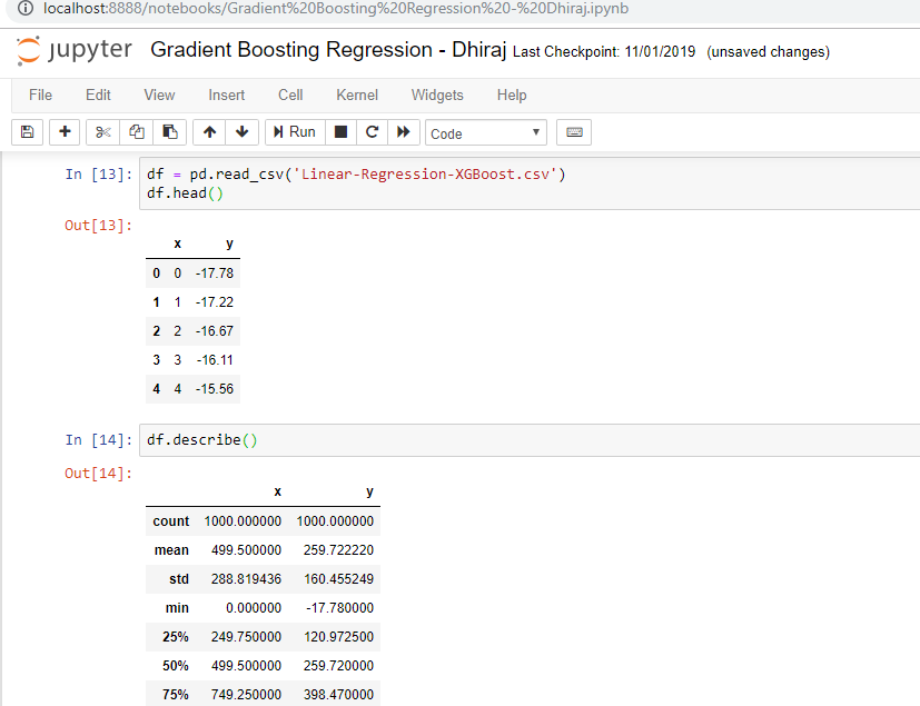
We are going to fit this data as a line whose equation will be like y = mx+c
The m is slope of the like and c is y intercept of the line.
Training the GBR model
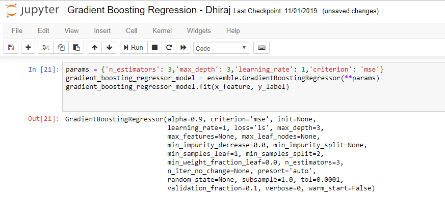
Its time to implement the model now. As you can see in the code below , we will start with defining the parameters n_estimators, max_depth, learning_rate and criterion. Values of these parameters are 3, 3, 1 and mse respectively. We have stored the parameter values in a variable called params.
We imported ensemble from sklearn and we are using the class GradientBoostingRegressor defined with ensemble.
We are creating the instance, gradient_boosting_regressor_model, of the class GradientBoostingRegressor, by passing the params defined above, to the constructor.
After that we are calling the fit method on the model instance gradient_boosting_regressor_model.
In cell 21 below you can see that the GradientBoostingRegressor model is generated. There are many parameters like alpha, criterion, init, learning rate, loss, max depth, max features, max leaf nodes, min impurity decrease, min impurity split, min sample leaf, mean samples split, min weight fraction leaf, n estimators, n iter no change, presort, random state, subsample, tol, validation fraction, verbose and warm start and its default values are displayed.
Evaluating the model
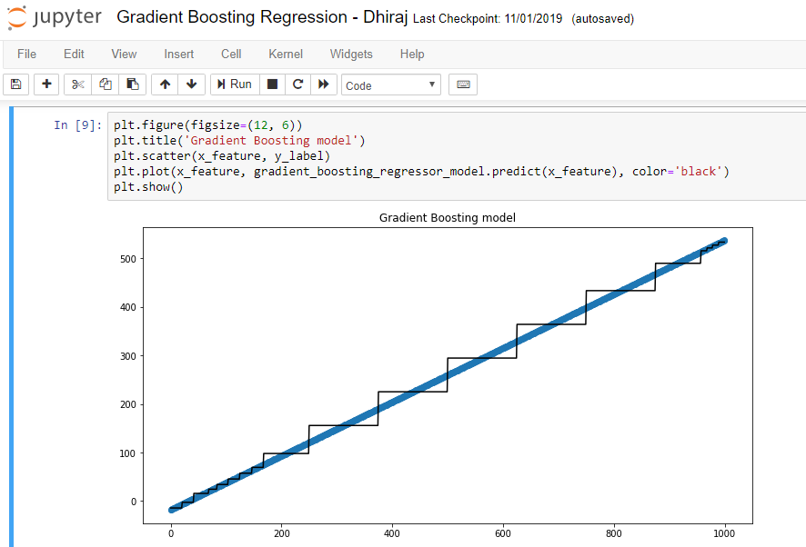
Let us evaluate the model. Before evaluating the model it is always a good idea to visualize what we created. So I have plotted the x_feature against its prediction as shown in the figure below. This gives us the better understanding of how well the model is fitting into the data. And as seen clearly from the diagram below, it looks like we have a good fit. We are using the pyplot library to create the below plot. As you can see in below code I have first set the figsize. After that using the title function we need to set the title of the plot. Then we need to pass the feature and label to the scatter function. And finally use the plot function to pass the feature , its corresponding prediction and the color to be used.
After the above visualization its time to find how best model fits the data quantitatively. sklearn provides metrics for us to evaluate the model in numerical terms.
As you can see below the fitment score of the model is around 98.90%. This is a really good score as expected from a model like Gradient Boosting Regression.

End Notes:
In this tutorial we learned what is Gradient Boosting Regression, what are the advantages of using it. We also discussed various hyperparameter used in Gradient Boosting Regression. After that we loaded sample data and trained a model with the data. With the trained model we tried to visualize and quantify how good the model is fitting into the data which is more than 98%.

Thanks for reading! Happy Machine Learning :)