
Time series analysis and forecasting have many applications: analyzing the sales of your retail chains, finding anomalies in the traffic you're getting to your servers, and predicting stock markets, to name a few.
There are diverse ways of digging into time series analysis. We will cover it with the following topics.
Bring this project to life
Table of Contents
- What Are the Properties of Time Series?
- Plotting Rolling Statistics
- Autocorrelation
- Partial Autocorrelation
- Seasonality
- Stationarity of a Time Series
- Tests for Stationarity
- ACF-PACF Plots
- Dickey Fuller Test
- KPSS Test
- Transformations for Stationarity
- Detrending
- Differencing
- Tests for Stationarity
- Conclusion
You can run the full code for this post for free from a Gradient Community Notebook.
Before we dive into the details of time series, let's prepare our dataset.
We will use weather data from Jena, Germany for our experiments. You can download it using the following command from the CLI.
wget https://storage.googleapis.com/tensorflow/tf-keras-datasets/jena_climate_2009_2016.csv.zipUnzip the file and you'll find CSV data that you can read using Pandas. The dataset has several different weather parameters recorded. For the purpose of this tutorial, we'll be using the temperature data (in Celsius). The data is recorded regularly; over 24 hour periods, with 10 minute intervals.
import pandas as pd
import matplotlib.pyplot as plt

df = pd.read_csv('jena_climate_2009_2016.csv')

time = pd.to_datetime(df.pop('Date Time'), format='%d.%m.%Y %H:%M:%S')
series = df['T (degC)']
series.index = time

print(df)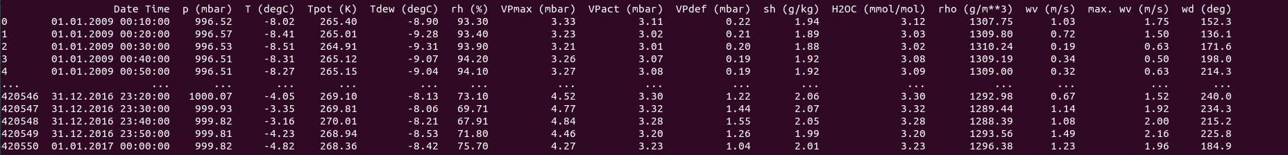
series.plot()
plt.show()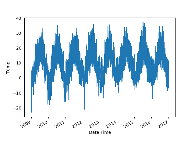
What Are the Properties of Time Series?
A time series is a sequence of observations taken sequentially in time. A certain variable varies along with time, and we analyze the patterns in it and try to make predictions based on the variations the series has shown in the past.
There are certain properties of a time series to look out for:
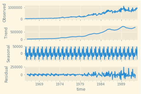
- Trends: An overall upward or downward movement in the variable over time.
- Seasonality: A periodic component to the time series, where a certain pattern repeats itself every few units of time.
- Residuals: The noisy components of a time series.
Decomposing a time series into these components can give us a lot of information and insight into how the time series behaves.
Rolling Statistics
The best way to start understanding a time series is by visualizing its rolling statistics. Let's plot the rolling statistics with a window of 2600 (monthly data, i.e. 30 days). You can also compare the rolling statistics with the mean value of the dataset, and the best fit line for all the data.
import numpy as np

plt.plot(series.index, np.array([series.mean()] * len(series)))

x = np.arange(len(series))
y = series.values
m, c = np.polyfit(x, y, 1)

plt.plot(series.index, m*x + c)

series.rolling(3600).mean().plot()

plt.legend(['mean', 'regression line', 'rolling mean'])
plt.ylabel('Temp')
plt.show()


roll_std = series.rolling(3600).std()
roll_std.dropna(inplace=True)
plt.plot(roll_std.index, np.array([roll_std.mean()] * len(roll_std)))

x = np.arange(len(roll_std))
y = roll_std.values
m, c = np.polyfit(x, y, 1)

plt.plot(roll_std.index, m*x + c)

roll_std.plot()
plt.legend(['rolling std mean', 'rolling std regression', 'rolling std'])
plt.ylabel('Temp')
plt.show()
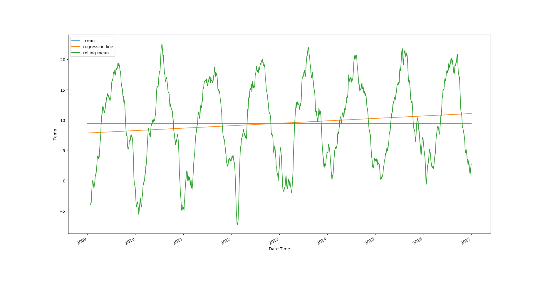
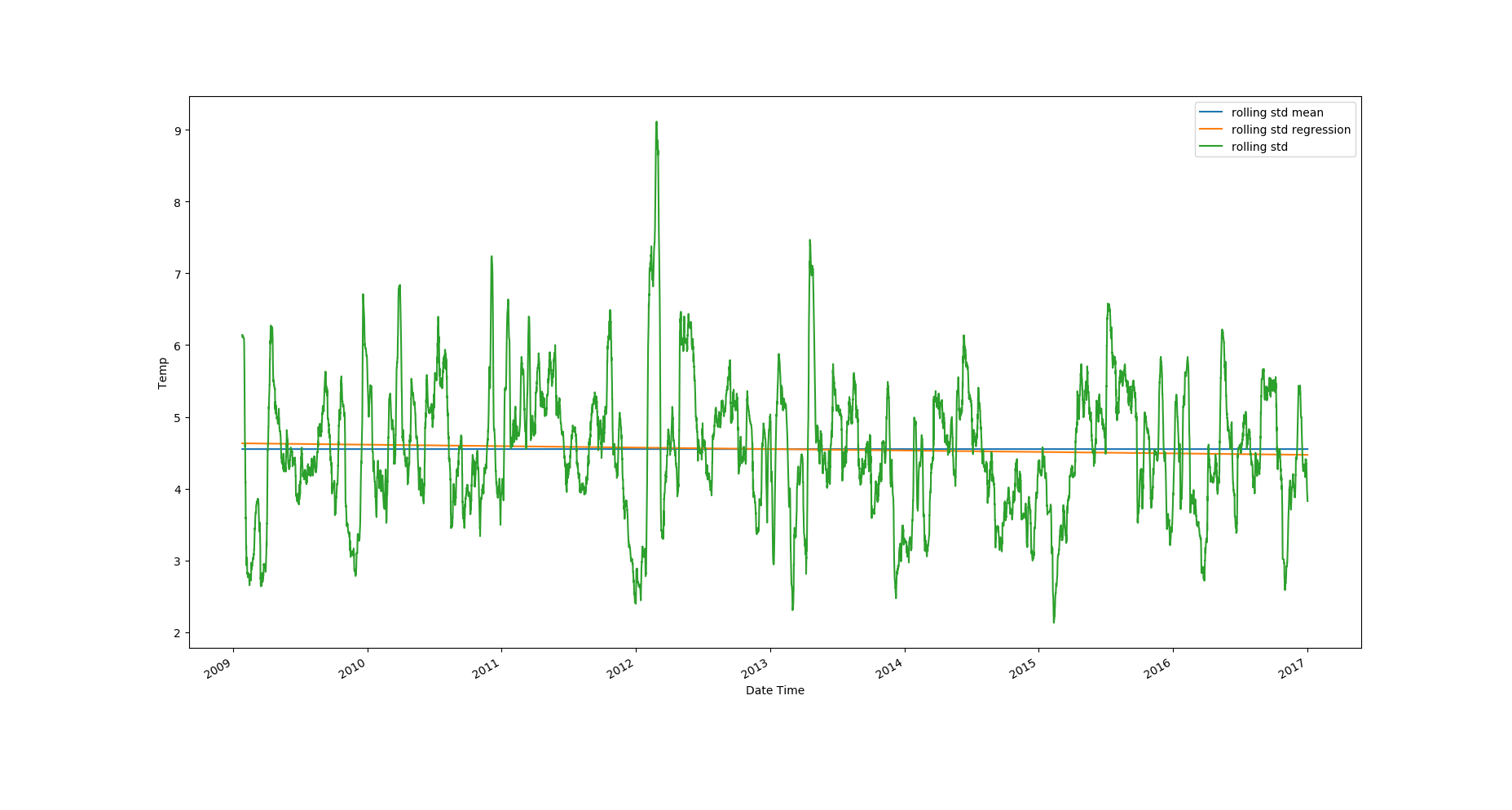
Looking at the plots, it's clear that the temperature values have an upward trend and there's strong seasonality in the data. The rolling standard deviation has a very weak downward trend, but the rolling standard deviation values themselves vary a lot.
Autocorrelation
We know that correlation lets us compare the relationship between two variables by assuming a Gaussian distribution, and using Pearson's coefficient to find the strength of the relationship between said variables.
The Pearson coefficient can be calculated as follows.
def correlation(x, y):
	x_norm = x - x.mean()
	y_norm = y - y.mean()
	return np.sum(x_norm * y_norm) / np.sqrt(np.sum(x_norm ** 2) * np.sum(y_norm ** 2))
Autocorrelation is the correlation of a signal with a delayed copy of itself as a function of delay. We try to find the correlation between a time series and a time lagged version of itself. We watch these values, and find how they vary as we increase the time lag. It can be calculated as follows.
def autocorrelation(x, k):
	val_0 = np.sum((x - x.mean()) ** 2) / len(x)
	val_k = np.sum((x[:-k] - x.mean()) * (x[k:] - x.mean())) / len(x)
	return val_k / val_0
Partial Autocorrelation
The partial autocorrelation function lets us calculate partial correlation between a time series and the same series with a time lag. The difference between correlation and partial correlation is that partial correlation lets us control the effect of other lag values.
The aim is to calculate the dependence of the same time series with different delays.
To find the dependence of all lag values with each other, we can formulate a linear equation of the following nature. Let $X(t - k)$ be a column vector of a time series with lag $k$. Our matrix generated above will then create an array of shape $(N \times k)$. Let's call it $A$. Now define another matrix with unknown coefficients $B$, which is of the same size as $X$.
Then we have a linear system of equations:
$X(t) = A \times B$
And we need to solve for $B$.
For lag values of 1 or 2 this is analytically simple to solve. That being said, it can get cumbersome pretty quickly.
Another way of approaching the problem is provided by the Yule Walker Equations. An element of a time series is represented as a linear equation dependent on each of its previous elements until the maximum lag value.
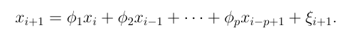
The equation is multiplied by the element at the maximum lagged time step and the expectation is calculated. The equation is divided by the length of the series, then by the zeroth autocovariance.
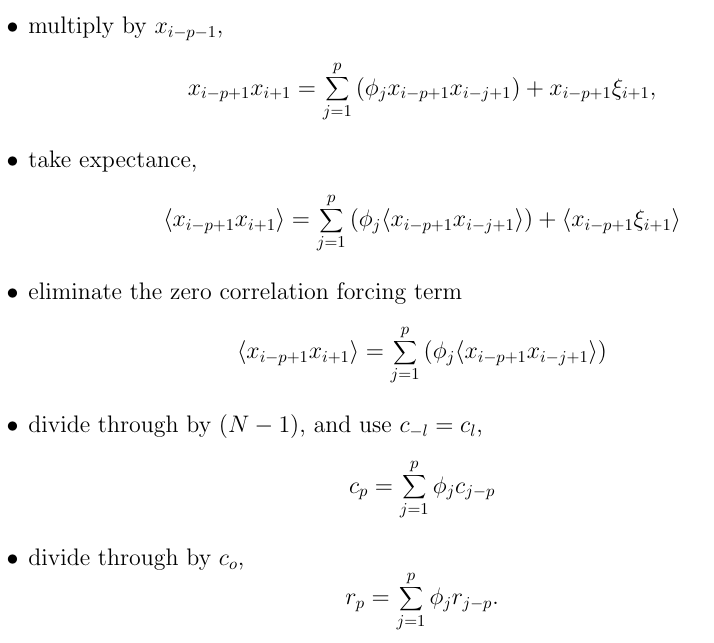
Here, $c(i)$ is the autocovariance value (which is divided by the zeroth value to get autocorrelation parameters $r(p)$).
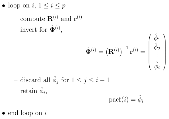
The equations for all the lag values can be neatly represented as follows.
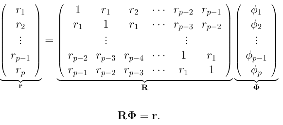
Now we need to solve for $\phi$. We know how to calculate the values of matrix $r$ from the autocorrelation function we defined. To find partial autocorrelations we can use out-of-the-box functions from the statsmodels package in Python, as follows.
from statsmodels.graphics.tsaplots import plot_acf, plot_pacf

def get_acf_pacf_plots(df):
    fig, ax = plt.subplots(2, figsize=(12,6))
    ax[0] = plot_acf(df, ax=ax[0])
    ax[1] = plot_pacf(df, ax=ax[1])


get_acf_pacf_plots(series[5::6])
plt.show()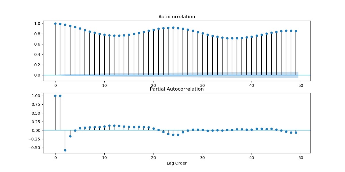
Seasonality
From several of our plots, we see that the data has a seasonal element to it. We know intuitively that the temperature data should have a seasonal component to it as well. The temperature should oscillate every day, lower during the nights compared to during the days. Besides that, they should also oscillate over the course of a year.
To validate these suspicions, we can look at the Fourier transforms of our series.
Fourier transforms allow us to make an amplitude-based series into a frequency-based series. They are complex-valued functions that represent every series as a superposition of sinusoidal waves in a complex plane.
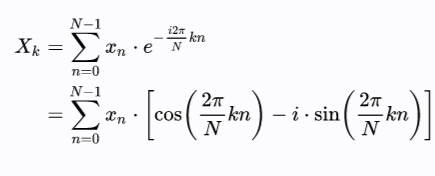
Here N is the length of the series, and X is the transformed value at t=k.
3Blue1Brown has done extremely interesting videos that will give you a very intuitive understanding of the mathematical formulation, why the values are represented in a complex plane, and how the dominant frequencies in a function are captured. You can find the video on Fourier series here and Fourier transforms here.
We can plot the magnitude of our Fourier transform as follows.
from scipy.fft import fft

fft_vals = fft(series[5::6].values)
f_per_dataset = np.arange(0, len(fft_vals))

n_samples_h = len(series[5::6])

hours_per_year = 24*365.2524
years_per_dataset = n_samples_h/(hours_per_year)

f_per_year = f_per_dataset/years_per_dataset
plt.step(f_per_year, np.abs(fft_vals))
plt.xscale('log')
plt.xticks([1, 365.2524], labels=['1/Year', '1/day'])
_ = plt.xlabel('Frequency (log scale)')
plt.show()
This snippet was borrowed from here.
We get the following plot:
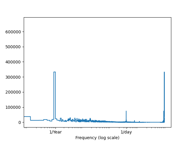
As we can see, the values around 1/Year and 1/Day show an unusual spike, validating our previous intuitions.
The above method is a basic form of spectral analysis. A lot of sophisticated methods for spectral density estimations have emerged which utilize the underlying idea of Fourier transforms: converting time domain information into the frequency domain. Some of them are Periodgrams, Barlett's Method, Welch's Method, etc. Often, to obtain better results, window functions like Hamming and Blackman-Harris are used to smooth the time series. You can think of these as 1-dimensional convolutional filters, where the parameters vary according to the kind of window function we are looking at. You can learn more about spectral analysis and Fourier transforms by reading up on digital signal processing.
Stationarity of a Time Series
A time series is stationary when its statistical properties like mean, variance, and autocorrelation don't change over time.
Methods like ARIMA and its variants work with the assumption that the time series they're modeling is stationary. If the time series is not stationary, these methods don't work very well.
Lucky for us, there are several tests we can do to determine if a time series is stationary. Even luckier for us, there are several transformations to convert a non-stationary time series to a stationary one, and back.
We will take a look at the tests first, and then the transformations.
ACF and PACF Plots
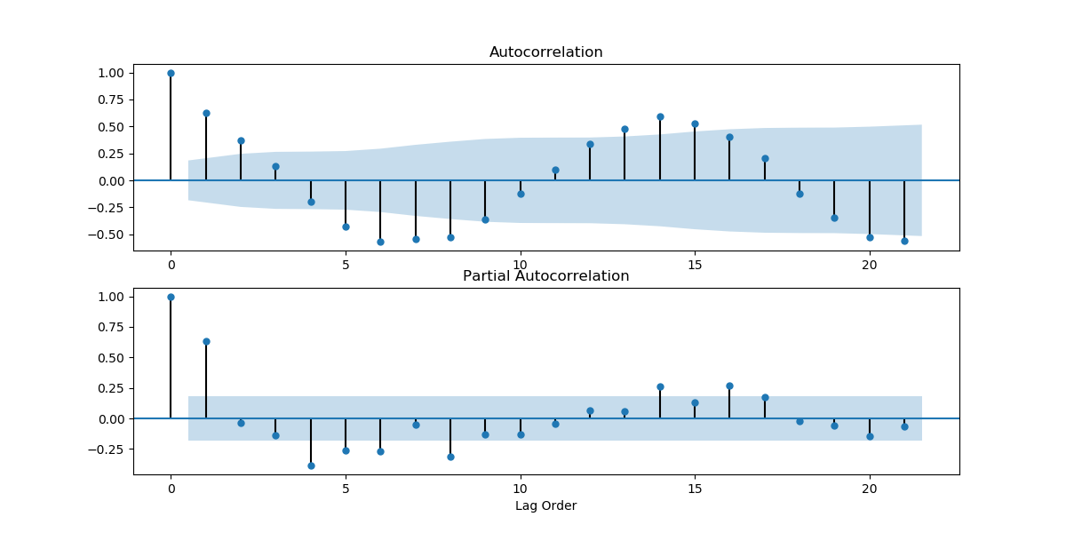
Looking at how the mean and variance of a time series changes over time can give us an initial idea of how non-stationary a time series is, and what kind of stationarizing mechanism can we apply. Looking at the plots we found above, we can guess that the weather time series is far from stationary. We can also look at the ACF and PACF plots. If the values on the plots fall quickly, chances are that the time series is close to stationary. But the ACF and PACF plots we got above were looking at values too close in time. The weather hardly changes every 10 minutes. Let's take a look at the plots when you take data by the day.
series2 = series[119::120]
get_acf_pacf_plots(series2)
plt.show()
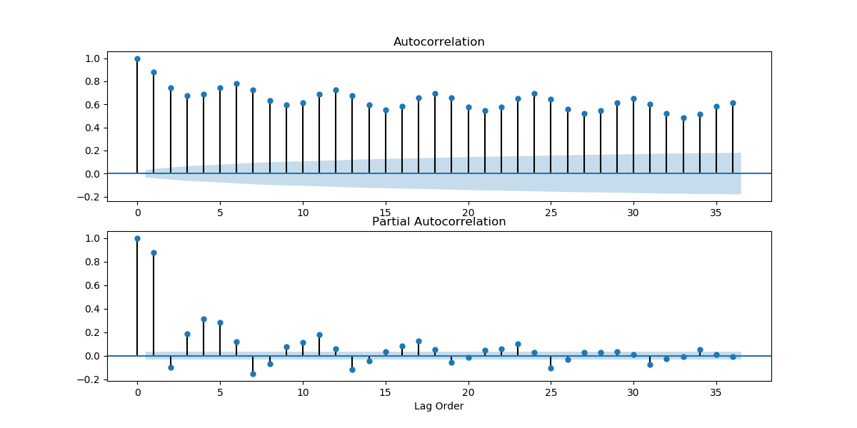
And if we took the data for every 31 days?
series2 = series2[30::31]
get_acf_pacf_plots(series2)
plt.show()
As we can see, there are several points that fall outside of the blue region, which indicates that the time series is not stationary.
Dickey-Fuller Test
Unit Root Tests test the null hypothesis that a unit root is present in an autoregressive model. The original test treats a time series as a lag-1 autoregressive model, and a unit root proves that a time series is not stationary.
There are three main versions of the test:
1. Test for a unit root:
$$ \Delta y_{t} = \delta_{y_{t-1}} + u_{t} $$
2. Test for a unit root with drift:
$$ \Delta y_{t} = a_{0} + \delta_{y_{t-1}} + u_{t} $$
3. Test for a unit root with drift and deterministic time trend:
$$ \Delta y_{t} = a_{0} + a_{1}t + \delta_{y_{t-1}} + u_{t} $$
The Augmented Dickey-Fuller Test is a one-tailed test that uses the same testing procedure, but applied to a lag-p series as shown below.

The lag value is found using information criterion like Akaike, Bayesian, or Hannan-Quinn.
from statsmodels.tsa.stattools import adfuller

def test_dickey_fuller_stationarity(df):
    dftest = adfuller(df, autolag='AIC')
    dfoutput = pd.Series(dftest[0:4], index=['Test Statistic',
                                             'p-value',
                                             'Number of Lags Used',
                                             'Number of Observations Used'])
    for key,value in dftest[4].items():
        dfoutput['Critical Value (%s)'%key] = value
    if dfoutput['Critical Value (1%)'] <  dfoutput['Test Statistic']:
        print('Series is not stationary with 99% confidence. ')
    elif dfoutput['Critical Value (5%)'] < dfoutput['Test Statistic']:
        print('Series is not stationary with 95% confidence. ')
    elif dfoutput['Critical Value (10%)'] < dfoutput['Test Statistic']:
        print('Series is not stationary with 90% confidence. ')
    else:
        print('Series is possibly stationary. ')
    return dfoutput

out = test_dickey_fuller_stationarity(series)
print(out)
The output we get is the following.
Series is possibly stationary.

Test Statistic                -8.563581e+00
p-value                        8.564827e-14
Number of Lags Used            6.200000e+01
Number of Observations Used    7.002800e+04
Critical Value (1%)           -3.430443e+00
Critical Value (5%)           -2.861581e+00
Critical Value (10%)          -2.566792e+00
You can learn more about the Augmented Dickey-Fuller Test here.
KPSS Test
Another unit root test is the KPSS test. Instead of assuming a null hypothesis of the presence of a unit root, the KPSS test considers it the alternative hypothesis. The following regression equation is used.
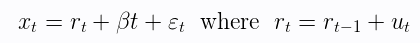
Where $r_t$ is a random walk, $\beta t$ is a deterministic trend, and $\epsilon_t$ is the stationary error.
The null hypothesis is thus stated to be H₀: σ² = 0, while the alternative is Hₐ: σ² > 0.
In the implementation we should remember that KPSS is a two-tailed test.
from statsmodels.tsa.stattools import kpss

def test_kpss(df):
    dftest = kpss(df)
    dfoutput = pd.Series(dftest[0:3], index=['Test Statistic',
                                             'p-value',
                                             'Number of Lags Used'])
    for key,value in dftest[3].items():
        dfoutput['Critical Value (%s)'%key] = value
    if abs(dfoutput['Critical Value (1%)']) < abs(dfoutput['Test Statistic']):
        print('Series is not stationary with 99% confidence. ')
    elif abs(dfoutput['Critical Value (5%)']) < abs(dfoutput['Test Statistic']):
        print('Series is not stationary with 95% confidence. ')
    elif abs(dfoutput['Critical Value (10%)']) < abs(dfoutput['Test Statistic']):
        print('Series is not stationary with 90% confidence. ')
    else:
        print('Series is possibly stationary. ')
    return dfoutput

out = test_kpss(series)
print(out)
And the output is the following.
Series is not stationary with 99% confidence.

Test Statistic            1.975914
p-value                   0.010000
Number of Lags Used      62.000000
Critical Value (10%)      0.347000
Critical Value (5%)       0.463000
Critical Value (2.5%)     0.574000
Critical Value (1%)       0.739000
There are several other tests you can do to test stationarity, like Phillip Herron, Zivot Andrews, Fourier ADF, etc., depending on how they treat structural breaks, endogenous and exogenous variables, etc. You can learn about them here and here.
Though unit root tests imply stationarity, there is a difference between unit root tests like Dickey-Fuller and stationarity tests like KPSS. You can learn more about it here and here.
Our time series has given us conflicting results. But if a series isn't stationary, stationarizing a time series is important because autoregressive models are designed with an underlying assumption of stationarity.
Transformations for Stationarity
There are a few different ways a time series can be made stationary.
1. Detrending
You can eliminate the trends in a time series by subtracting the rolling mean values from the series and then normalizing it.
def eliminate_trends(series):
    roll = series.rolling(4).mean()
    avg_diff = (series - roll)/roll
    avg_diff.dropna(inplace=True)
    return avg_diff


diff = eliminate_trends(series[5::6])
test_dickey_fuller(diff)
test_kpss(diff)
Dickey-Fuller results:
Series is possibly stationary.

Test Statistic                  -264.739131
p-value                            0.000000
Number of Lags Used                0.000000
Number of Observations Used    70087.000000
Critical Value (1%)               -3.430443
Critical Value (5%)               -2.861581
Critical Value (10%)              -2.566792
KPSS results:
Series is possibly stationary.

Test Statistic            0.302973
p-value                   0.100000
Number of Lags Used      62.000000
Critical Value (10%)      0.347000
Critical Value (5%)       0.463000
Critical Value (2.5%)     0.574000
Critical Value (1%)       0.739000
If you find a linear trend in the series, you can instead find the regression line and then remove the linear trend accordingly.
def eliminate_linear_trend(series):
    x = np.arange(len(series))
    m, c = np.polyfit(x, series, 1)
    return (series - c) / m

diff = eliminate_linear_trend(series[5::6])
test_dickey_fuller(diff)
test_kpss(diff)
Dickey-Fuller:
Series is possibly stationary.
Test Statistic                   -42.626441
p-value                            0.000000
Number of Lags Used               62.000000
Number of Observations Used    84045.000000
Critical Value (1%)               -3.430428
Critical Value (5%)               -2.861574
Critical Value (10%)              -2.566788
KPSS:
Series is possibly stationary.

Test Statistic            0.006481
p-value                   0.100000
Number of Lags Used      65.000000
Critical Value (10%)      0.347000
Critical Value (5%)       0.463000
Critical Value (2.5%)     0.574000
Critical Value (1%)       0.739000
2. Differencing
You can pick a lag value and difference the value at time $t$ with the value at time $t - p$, where $p$ is the lag value.
def difference(series, lag=1):
	differenced = []
    for x in range(lag, len(series)):
    	differenced.append(series[x] - series[x - lag])
    return pd.Series(differenced)
After differencing, we can try the Dickey-Fuller and KPSS tests again.
diff = difference(series[6::5])
test_dickey_fuller(diff)
test_kpss(diff)
Outputs from Dickey-Fuller:
Series is possibly stationary.

Test Statistic                   -42.626441
p-value                            0.000000
Number of Lags Used               62.000000
Number of Observations Used    84045.000000
Critical Value (1%)               -3.430428
Critical Value (5%)               -2.861574
Critical Value (10%)              -2.566788
And KPSS:
Series is possibly stationary.

Test Statistic            0.006481
p-value                   0.100000
Number of Lags Used      65.000000
Critical Value (10%)      0.347000
Critical Value (5%)       0.463000
Critical Value (2.5%)     0.574000
Critical Value (1%)       0.739000
Conclusion
We covered all the basics of what to look for in a time series to analyze linear and nonlinear trends. We looked into the concept of stationarity, different tests to find out if a series is stationary, and how to stationarize a non-stationary series. In the next part of this series we will cover time series forecasting.
Don't forget to run the full code for this post for free from a Gradient Community Notebook, or check out Parts 2 and 3 covering regression and LSTMs, and autoregressive models and smoothing methods, respectively.