
This is Part 2 of our series on Reinforcement Learning (RL) concepts for folks who already have some experience with machine learning. In Part 1, we primarily focused on Markov Decision Processes (or MDPs), the mathematical framework used to model problems in Reinforcement Learning.
In this part, we will be taking a brief tour of the RL universe, covering things like the basic jargon, similarities and dissimilarities between RL and other forms of machine learning, the anatomy of an RL algorithm, and much more.
This part assumes familiarity with Markov Decision Processes (MDPs), which we have covered extensively in Part 1. If you aren't familiar with MDPs or need a refresher, I strongly recommend going through Part 1 before continuing with this article.
Here are the things that we will cover in this post.
Bring this project to life
- Why Reinforcement Learning? Why Not Supervised Learning?
- Optimizing the Reward Function
- Supervised Learning With Labels
- Distribution Shifts
- Anatomy of an RL Algorithm
- Collecting the Data
- Off-Policy vs On-Policy
- Exploration vs Exploitation
- Why Off-Policy?
- Why On-Policy?
- Computing the Return
- Estimating the Expected Return in Model-Free Settings
- Discount Factor
- Value Functions
- N-Step Returns
- Updating the Policy
- Q-Learning
- Policy Gradients
So, let's get started.
Why Reinforcement Learning? Why Not Supervised Learning?
The central goal of reinforcement learning is to maximize the cumulative reward, or the return. In order to do this, the agent should find a policy $ \pi(s) $ which predicts an action $ a $, given state $ s $, that maximizes the return.
Optimizing the Reward Function
Just like we minimize a loss function using gradient descent in standard ML, can we maximize the returns using gradient ascent too? (Instead of finding the minima, gradient ascent will converge on the maxima.) Or is there a problem?
Consider a mean-squared loss for a regression problem. The loss is defined by:
$$ L(X,Y;\theta) = \frac{1}{2}(Y - \theta^TX) ^ 2 $$
Here $ Y $ is the label, $ X $ is the input, and $ \theta $ are the weights of the neural network. The gradient of this can be easily computed.
On the other hand, the return is constructed by adding the rewards. The rewards are generated by the environment's reward function, which may not be known to us in many cases (model-free settings). We can't compute a gradient if we don't know the function. So, this approach won't work!
Supervised Learning With Labels
If the reward function is not known to us, maybe what we can do is construct our own loss function which basically penalizes the agent if the action taken by the agent is not the one that leads to the maximum return. In this way, the action predicted by the agent becomes the prediction $ \theta^TX$ and the optimal action becomes the label.
For determining the optimal action at each step, we require an expert human/software. Examples of work done in this direction include Imitation Learning and Behavioural cloning where the agent is supposed to learn using demonstrations by an expert (head to further reading for links on these).
However, the number of demonstrations/labeled data required for such an approach may prove to be a bottleneck for good training. Human labeling is an expensive business and given how data-hungry deep learning algorithms tend to be, collecting so much expert labeled data may not be feasible at all. On the other hand, if one has a piece of expert software, then one needs to wonder why to build another piece of software using AI for solving a task for which we already have expert software!
Furthermore, approaches that use expert trained data for supervision are often limited by the upper bound of the expertise of the expert. The policy of the expert may just be the best available at the moment, not the optimal one. We would ideally like the RL agent to discover the optimal policy (which maximizes the return).
Also, such approaches would not work for unsolved problems for which we don't have experts.
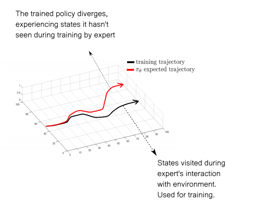
Distribution Shifts
Another issue with solving problems with expert-labelled data are distribution shifts. Let us consider the case of an expert agent playing SeaQuest, a game where you have pick up divers from under the sea. The agent has a depleting source of oxygen and has to routinely go to the surface to recollect oxygen.

Now assume that the expert agent's policy never leaves the agent in a state where oxygen is less than 30%. Therefore, no data collected by following this policy would have states where the oxygen is below 30%.
Now imagine an agent is trained from the dataset created using the above expert's policy. If the trained agent is imperfect (100% performance is unrealistic) and finds itself in a state where oxygen is about 20%, it may not have experienced the optimal actions to be taken in such a state. This phenomenon is called a distribution shift and can be understood using the diagram below.
One famous work in imitation learning that has been used to combat distribution shifts Dagger, a link to which I have provided below. However, this approach was also marred by high data acquisition costs both in terms of money and time spent.
The Anatomy of an RL Algorithm
In RL, instead of learning using labels, the agent learns through trial and error. The agent tries out a bunch of things observing what fetches a good return and what fetches a bad return. Using various techniques, the agent comes up with a policy that is supposed to execute actions that give maximum or close to maximum returns.
RL algorithms comes in all shapes and sizes but most of them tend to follow a template which we here refer as the Anatomy of a RL algorithm.
Any RL algorithm, in general, breaks the learning process into three steps.
- Collect the data
- Estimate the return
- Improve the policy.
These steps are repeated multiple times until the desired performance is reached. I am refraining to use the word convergence because for many Deep RL algorithms, there are no theoretical guarantees of convergence, just that they seem to work well in practice for a wide range of problems.
The rest of this article will be about going into depth into each of the above.
Collecting the Data
Unlike a standard machine learning setting, there is no static dataset in RL settings over which we can iterate repeatedly to improve our policy.
Instead, we have to collect the data by interacting with the environment. The policy is run and the data is stored. Data is generally stored as a 4-tuple values $ \langle s_t, a_t, r_t, s_{t+1} \rangle $ where,
- $ s_t $ is the the initial state
- $ a_t $ is the action taken
- $ r_t $ is the reward accrued as a result of taking $ a_t $ in $ s_t $
- $ s_{t+1} $ is the new state agent transitions to as a result of taking $ a_t $ in $ s_t $
Off-Policy vs On-Policy
RL algorithms often alternate between collecting data and improving the policy. The policy that we use to collect the data maybe different from the policy which we are training. This is called Off-Policy Learning.
The policy which collects the data is called the Behavioural policy, while the policy which we are training (which we plan to use using test time) is called the Target Policy.
In an alternate setting, we might use the same policy which we are training to collect the data. This is called On-Policy Learning. Here the Behavioural policy and the target policy are the same.
Let us understand the distinction between the help of an example. Consider we are training a target policy which gives us an estimated return for each action (consider actions to be discrete), and we have to chose the action that maximizes this estimate. In other words, we act greedily with respect the the action score.
$$ \pi(s) = \underset{a \in \mathcal{A} }{\arg\max} R_{estimate}(a) $$
Here, $ R_{estimate} $ is the return estimate.
During the data collection phase, we chose random actions to interact with the environment, disregarding return estimates. When we update our target policy, we assume that the trajectory taken by the policy beyond $ \langle s_t, a_t, s_{t+1} \rangle $ would be determined by choosing actions greedily w.r.t to estimated return. In contrast, when we collect the data, we pick random actions.
Therefore, our behavioural policy is different from our training one i.e. the greedy policy. This is therefore off-policy training.
If we use the greedy policy for data collection as well, this would become an on-policy setting.
Exploration vs Exploitation
Apart from the credit assignment problem, this is the one of THE biggest challenge in RL; so much so that guarantees it's own post, but I will try to give a brief overview here.
Again let us take an example. You are a data scientist who writes production grade code. You write NumPy code using vectorisation wherever possible. Now, you have this really important project coming your way which you totally want to nail.
You think to yourself, whether I should continue making rigorous use of vectorisation in my code to optimise it? Or should I devote some time to add more techniques like broadcasting and reshaping to my arsenal to write even more optimised code that is possible through just vectorisation. If you are thinking in that direction, you can head to our extensive 4-part series on NumPy Optimisation that covers all of these things mentioned above and much more!
 Ayoosh Kathuria
We have all been in such situations before. Is my current workflow good enough, or should I explore Docker? Is my current IDE good enough, or should I learn Vim? All these scenarios are basically choices between whether we want to explore more in pursuit of new tools, or exploit the knowledge we currently have!
In the world of RL algorithms, the agent starts out by exploring all behaviours. In due course of training, through trial and error, it recognises to some extent what works and what doesn't.
Once it gets to a decent level of performance, should it exploit what it has learnt, as the training further goes on to become better? Or should it explore more to maybe discover new methods of maximising the return. This is what is at the heart of the exploration v/s exploitation dilemma.
The RL algorithm must balance both in order to ensure good performance. The best solution lies somewhere in middle of totally exploratory and exploiting behaviours. There are multiple ways the balance of these behaviours is baked into the data collection policies.
In an off-policy setting, the data collection policy maybe totally random leading to overly exploratory behaviour. Alternatively, one can take a step according to the training policy or take a random action randomly with some probability. This is a popularly used technique in Deep RL.
p = random.random()

if p < 0.9:
	# act according to policy
else:
	# pick a random action
In on-policy settings, we can perturb the actions using some noise, or predict the parameters of a probability distribution and sample from it to determine what actions to take.
Why Off-Policy?
The biggest advantage of off policy learning that it helps us with exploration. The target policy can turn very exploitative in nature, not explore the environment well enough and settle for a sub-optimal policy. A data collection policy that is exploratory in nature will deliver diverse states from the environment to the training policy. For this reason, the behavioural policy is also called the exploratory policy.
Additionally, off-policy learning allows the agent to use data from older iterations whereas for on-policy learning, new data has to be collected every iteration. However, if the data collection operation is expensive, then on-policy may increase computational time of the training process.
Why On-Policy?
If off-policy learning is so great at encouraging exploration, why do we even want to use on-policy learning? Well, the reason has to do a bit with the mathematics of how the policy is updated (step 3).
With off-policy updates, we are basically updating the behaviour of the target policy using trajectories generated by another policy. Given similar set of initial states and action, our target policy could have led to different trajectories and returns. If these diverge too much, the updates can modify the policies in unintended ways.
It is for this reason we don't always go for off-policy learning. Even when we do, the updates only work well when the difference between two policies ain't very large, therefore, we sync our target and behavioural polices periodically and use techniques like importance sampling when making off-policy learning updates. I leave the discussion on the fine maths and importance sampling to another post.
Computing the Return
The next part in the learning loop for RL algorithms is computing the return. The central goal of Reinforcement Learning is to maximise the expected cumulative reward, or simply the return . The word expected basically factors in the possible stochastic nature of policy as well as the environment.
When we are dealing with cases where the environments are episodic in nature (i.e. an agent's life terminates eventually. Like a game such as Mario, where the agent can finish the game, or die by falling / getting bitten), the return is termed as a finite-horizon return. In case where are dealing with continuing environments (no terminal state), the return is termed as an infinite-horizon return.
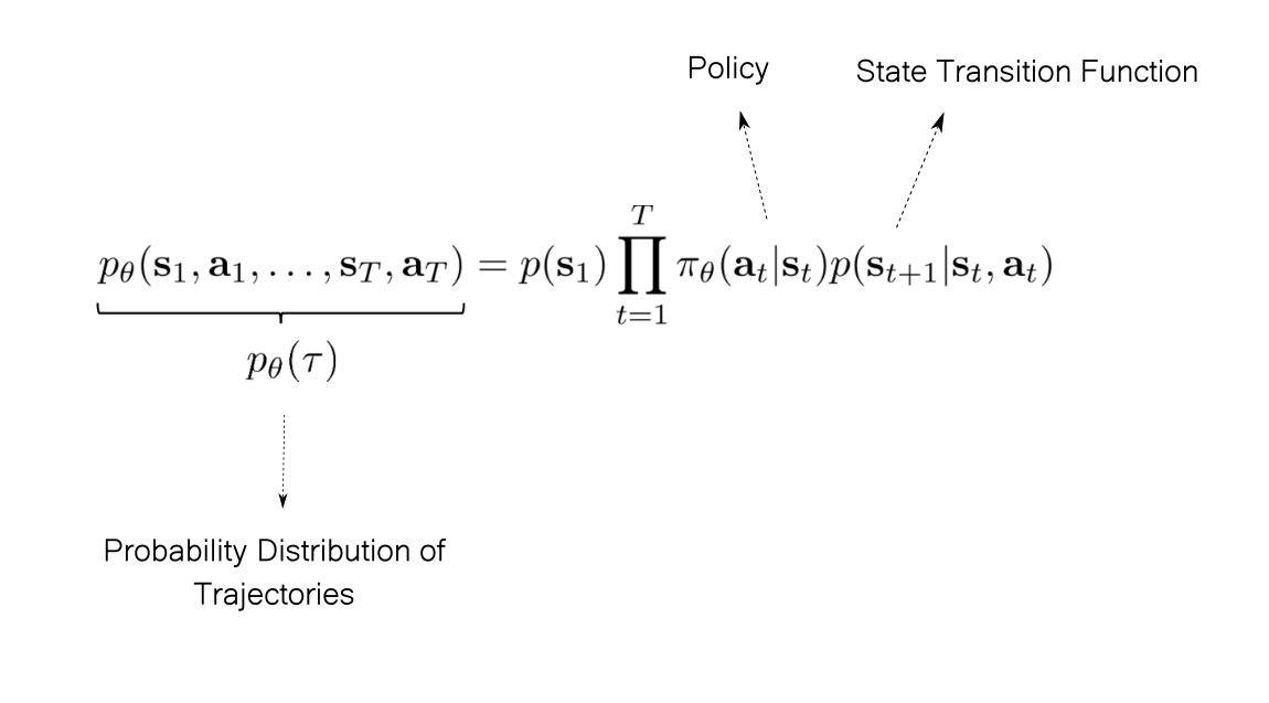
Let us only consider episodic environments. Our policy might be stochastic, i.e. given a state $ s $, it may take different trajectories $ \tau $ to the terminal state, $ s_T $.
We can define a probability distribution over these trajectories using
- Policy (which gives us the probabilities of various actions), and
- The state transition function of the environment (which gives us the distribution of future states given state and action).
The probability of any trajectory starting from an initial state $ s_1 $ and ending in a terminal state $ s_T $ is given by
Once we have the probability distribution over trajectories, we can compute the expected return over all possible trajectories as follows.
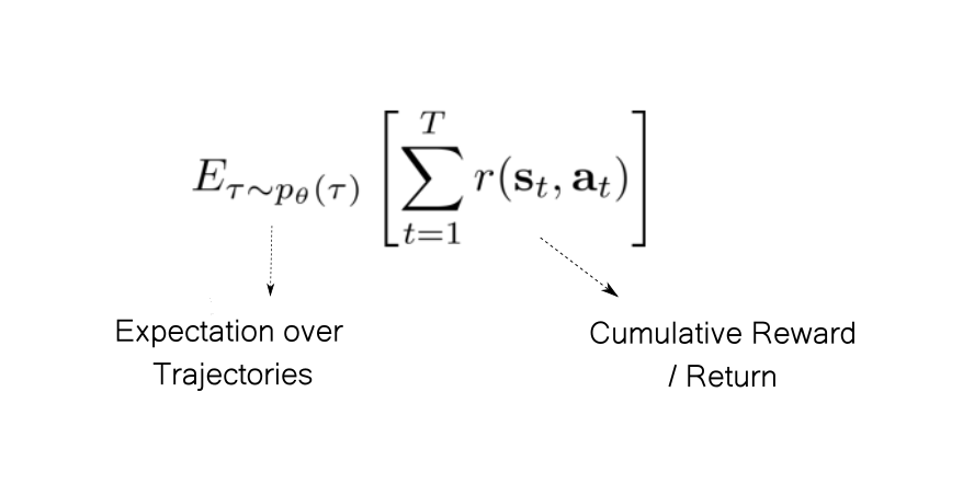
It is this quantity that RL algorithms are designed to maximise.
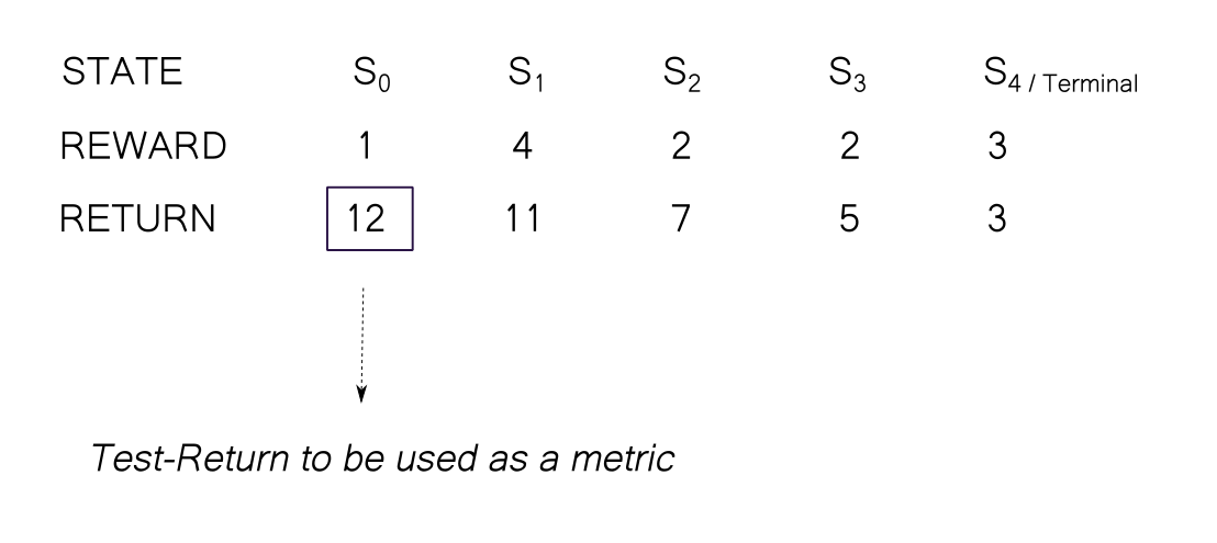
Note that it is very easy to get confused between reward and return. The environment provides the agent a reward for every single step whereas return is the sum of these individual rewards.
We can define return $ G_t $ at the time $ t $ as the sum of rewards from that time.
$$ G_t = \sum_{t}^{T} r(s_t, a_t) $$
Generally, when we talk about maximising the expected return as an objective of solving the RL task, we talk about maximising $ R_1 $ i.e. the return from the initial state.
Mathematically, we optimise the algorithms to maximise every $ R_t $. If the algorithm is able to maximise every $ R_t $, then $ R_1 $ gets automatically maximised. Conversely, it's absurd to try maximise $ R_{1...t-1} $ using action taken at time $ t $. The policy can't alter actions taken previously.
To differentiate $ R_1 $ return from the general return $ R_t $, we will call the former the test return and latter, just the return.
Estimating The Expected Return In Model-free Settings
Recall from the last post that a lot of times we try to directly learn from experiences and we have no access to state transition function. Such settings are a part of Model-free RL. In other cases, the state space may be so large that computing all the trajectories is intractable.
In such cases, we basically run the policy multiple times and average the individual returns to get an estimate value of return. The following expression estimates the expected return.
$$ \frac{1}{N} \sum_{i}^{N} \sum_{t} ^ {T} r(s_{i,t} , a_{i,t}), $$
where $ N $ is the number of runs, and $ r(s_{i,t} , a_{i,t}) $ is the reward got obtained at time $ t $ in the $ i^{th} $ run
The more the number of runs we do, the more accurate will our estimate be.
Discount Factor
There are a couple of problems with the above formulation for the expected return.
- In the case of continuing tasks where there is no terminal state, the expected return is an infinite sum. Mathematically, this sum may not converge with an arbitrary reward structure.
- Even in the finite horizon case, the return for a trajectory consists of all the rewards starting a state, say, $ s $ all the way up the terminal state $ s_T $. We weigh all the rewards equally, irrespective of whether they occur sooner or much later. That is quite unlike how things work in real life.
The second point basically asks the question "Is it necessary to add all the future rewards while calculating the return?" Maybe we can do with only the next 10 or 100? That will also solve the problem arising with continuing tasks since we don't have to worry about infinite sums.
Consider you are trying to teach a car how to drive through RL. The car gets a reward between 0 and 1 for every time step depending upon how fast it's going. The episode terminates once we have clocked 10 minutes of driving or earlier in case of collision.
Imagine the car gets too close to a vehicle and must slow down to avoid a collision and termination of the episode. Note that collision might still be a few time steps away. Therefore, until the collision happens, we will still be getting rewards for high speed before the car crashes. If we just consider only immediate or the 3 immediate returns for the reward, then we will be getting a high return even when we are on the collision course!
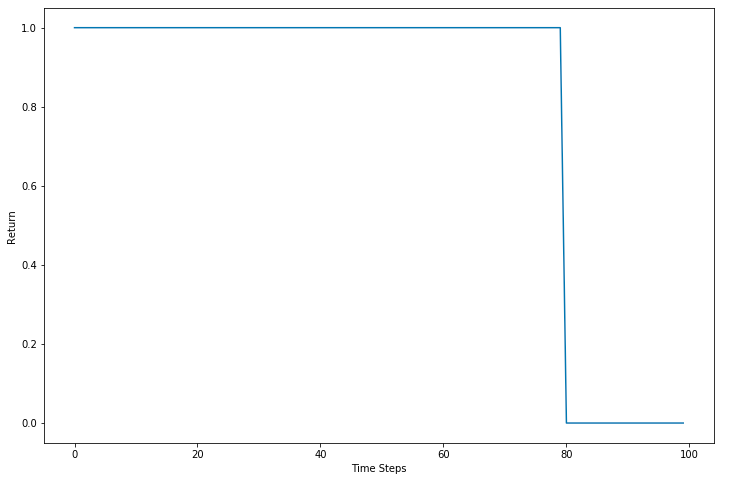
Suppose, the 10-minute episode is divided into 100 time steps. The car goes at full speed till 80 time steps and 0 afterward since it collides at the 80th time step. Ideally, it should have slowed down to avoid the collision.
Let's now use the future three rewards to compute the return.
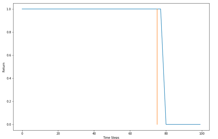
The orange line represents the 75 time-step mark. The vehicle should at least start to slow down here. In other words, the return should be less so such behaviors (speed on a collision path) are discouraged. The return starts to fall only after the 78th time step when it's too late to stop. The return for speeding at the 75th time step should be less too.
We want returns that incentivize foresight. Maybe we should add more future rewards to compute our returns.
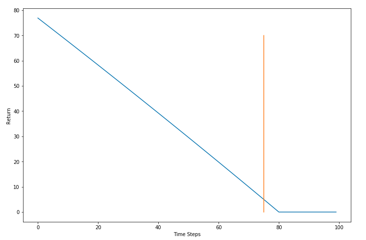
What if we add all the future returns like in the original formulation. With that, our return keeps falling as we move forward, even during time steps 1-50. Note that actions taken during T = 1-50 have little to no effect on the actions that led to the collision at T = 80.
The sweet spot lies somewhere in between. For doing this, we introduce a new parameter $ \gamma $ that does exactly that. We rewrite our expected return as follows.
$$\frac{1}{N} \sum_{i}^{N} \sum_{t = t'} ^ {T} \gamma^{t - t'} r(s_{i,t} , a_{i,t}) $$
Here is how the discounted return $ G_1 $ looks like.
$$ G_1 = r_1 + \gamma r_{2} + \gamma^2 r_3 + \gamma ^ 3 r_4 + ... $$
This is often termed as discounted expected return. $ \gamma $ is called the Discount Factor
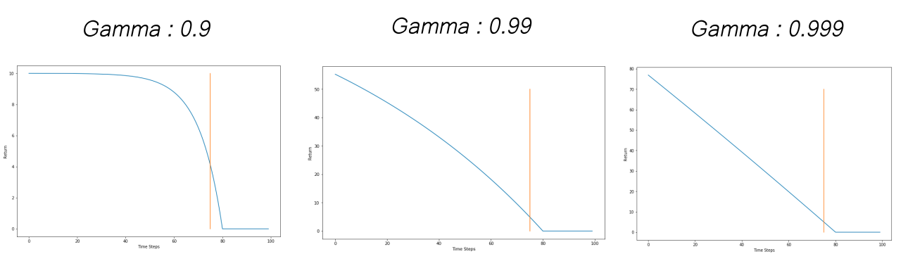
The parameter $ \gamma $ lets us control how far we are looking into the future when it comes to using rewards to compute our return. A higher value of $ \gamma $ will have us look further into the future. The value of $ \gamma $ is between 0 and 1. The weightage of the rewards fall exponentially with each time step. Popular values used in practice are 0.9, 0.99 and 0.999. The following graph shows how $ \gamma $ effects the return for our car example.
Under reasonable assumptions, discounted infinite sums can be shown to converge, which makes them useful in cases of continuing environments with no terminal state.
Value Functions
While we can define compute the discounted returns in the way mentioned above, here is a catch. Computing such a return for any state will require you to complete the episode first or carry out a large number of steps before you can compute the return.
Another way to compute the returns is to come up with a function, that takes the state $ s $ and the policy $ \pi $ as the input and estimates the value of the discounted return directly, rather than us having to add up future rewards.
The value function for a policy $ \pi $ is written as $ V^\pi (s)$. Its value is equal to the expected return if we were to follow the policy $ \pi $ starting from state $ s $. In RL literature, the following notation is used to describe the value function.
$$ V^\pi(s) = \mathbb{E} [ G_t | S_t = s] $$
Note that we don't write $ G_t $ as a function of the state and the policy. This is because we treat $ G_t $ just as sum of rewards returned from the environment. We have no clue (in model-free settings) how these rewards are computed.
However, $ V^\pi(s ) $ is a function that we predict ourselves using some estimator like a neural network. There, it's written as a function in the notation.
A slight modification of the value function is the Q-Function which estimates the expected discounted return if we take an action $ a $ in the state $ s $ under policy $ \pi $.
$$ Q^\pi(s,a) = \mathbb{E} [ G_t | S_t = s, A_t = a] $$
The policy that maximises the value function for all states is termed as the optimal policy.
There are quite a few ways how value functions are learned in RL. If we are in a model-based RL environment and the state space is not prohibitively large, then we can learn value functions through dynamic programming. These methods use recursive formulations of value functions, known as the Bellman Equations to learn them. We will cover Bellman Equations in-depth later in a post on Value Function Learning.
In the case where the state space is too large, or we are in a model-free setting, we can estimate the value function using supervised learning where labels are estimated by averaging many returns.
N-Step Returns
We can mix returns and value functions to arrive at what are called n-step returns.
$$ G^{n}_t = r_{t} + \gamma r_{t+1} + ... +\gamma ^{n-1} r _ {t + n - 1} + \gamma ^ 3 V(s_{t+n}) $$
Here is an example of 3-step return.
$$ G^{3}_t = r_{t} + \gamma r_{t+1} + \gamma^2 r_{t+2} + \gamma ^ 3 V(s_{t+3}) $$
In literature, using the value functions for computing the rest of the return (that come after n-steps) is also called as Bootstrapping.
Updating the Policy
In the third part, we update the policy so that it takes actions which maximise the Discounted Expected Reward (DER)
There are a couple of popular ways to learn the optimal policies in Deep RL. Both of these approaches contain objectives that can be optimised using Backpropagation.
Q-Learning
In Q-Learning, we learn a Q-function and pick actions by acting greedy w.r.t to the Q-values for each action. We optimise a loss with an aim to learn the Q-function.
Policy Gradient
We can also maximise the expected return by performing gradient ascent on it. The gradient is called the policy gradient.
In this approach, we directly modify the policy so that actions that led to more rewards in experience collected are made more likely, while the actions that led to bad rewards are made less likely in the probability distribution of the policy.
Another class for algorithms called Actor-Critic algorithms combines Q-Learning and policy gradients .
Conclusion
This is where we conclude this part. In this part, we covered the motivation for using RL methods and the basic anatomy of RL algorithms.
If you feel that I didn't give enough attention to the last section, i.e. the one on updating the policy, that's fair due. I kept the section short because each approach mentioned merits its own post(s)! In the coming weeks, I will be writing dedicated blog posts for each of these approaches, along with code that you can run. Till then, codespeed!