Missing data is a situation where there are no observations for certain instances, like rows, in a dataset. This is usually problematic for predictive modeling, as less information means less distribution and precision in estimating relationships in the data.

Most practitioners stick to the common, traditional techniques of handling all forms of missing data, despite their apparent faults in certain scenarios, mostly due to unfamiliarity with superior techniques and the difficulty in implementing them.

There are others, who entirely object to missing data imputation for predictive modeling, as they consider it a form of generating artificial data. These objections are, often, unfounded because predictive modeling is aimed at estimating relationships between variables to make accurate predictions, and imputation aims to reduce the bias in models by imputing values that model the information that missing values would provide. Moreover, missing data imputation has consistently produced better results as compared to deletion (source).

When handling missing data, which we will refer to as absence of data, it is important to understand the missing data pattern. This is helpful to show the kind (random or systematic) and the extent (considerable or negligible) of the missing data.

Understanding the mechanism behind data absence is helpful in determining the specific methods to implement in handling such absence. There are certain assumptions on the general mechanism for missing data. While we can only theorize about why missing data may occur, these distinctions are useful in choosing efficient approaches to handling such occurrences.

Assumptions for Missing Data Mechanisms

1. Missing Completely At Random (MCAR): The data is Missing Completely At Random if the probability of missing values in a variable does not depend on any other variable in the data. This means that the absence does not follow any defined pattern and the probability of absence is uncorrelated with the observed data but results from a completely random process.
2. Missing At Random (MAR): This assumes that absence in a variable is related to some other observed variables in the data. This means that values are missing due to the values of certain observed variables. In MAR, there is a defined pattern of absence according to the observed data and a subset of the data that is affected by the observed variable is likely to be missing. It is important to note that the values in MAR are missing due to other observed variables, and not because of the nature of its own values.
3. Missing Not At Random (MNAR): This assumes that absence is due to variables that are not captured in the data. This refers to situations when the missing data occurs in a way that we cannot fully account for through observed data. This is often the most problematic absence of data to detect and handle.

To further differentiate between these mechanisms, let’s assume a dataset with the IQ and performance score of students in a test, with missing values in the performance score variable.

The absence is MCAR if the test scores are neither missing because of the values of the IQ ( i.e there are missing scores for students with both low and high IQs) nor are they missing because of the values of the scores themselves (i.e both high and low test scores are missing).

The absence is MAR if test scores are missing because of the observed IQ (e.g The students with low IQ are not interested in taking the test or recording their scores).

The absence is MNAR if the missing test score is due to the particular score of certain students in the test (e.g The students with low test score not recording their performances, regardless of whether their IQs are high or low).

Oftentimes, practitioners apply random techniques to handle absence in their data, without first understanding the mechanism behind such absence. This is an erroneous practice as common handling techniques don't efficiently handle MAR and MNAR scenarios and introduce bias when used as such.

In the following section, we will compare the performances of missing data handling techniques on a MAR data scenario and try to understand the reasons behind their performances.

The Dataset

We are going to be simulating a Missing At Random scenario from a complete dataset, so we can compare the results of the original dataset with those from applying handling techniques.

We will be using the Energy Efficiency Dataset. The study looked into assessing the heating load and cooling load requirements of buildings based on the building's parameters. The dataset contains 768 samples and 8 features, aiming to predict two real-valued responses ( The Heating Load and The Cooling Load). In our case, we will be comparing the performances in predicting the Heating Load.

For simplicity and to easily distinguish the real effects of these techniques on the MAR dataset, we will not be applying feature engineering or selection to the dataset. These are highly recommended to further improve the performance of machine learning models, but not within the scope of this analysis.

Loading The Dataset

We load the dataset and remove the 'Cooling Load' variable that we don't need. We also split the dataset into train and test sets to properly evaluate our model's performance.

# import required libraries
import pandas as pd
import numpy as np
from sklearn.model_selection import train_test_split

# load the dataset
# remove unwanted columns
data = pd.read_csv('energy_efficiency_data.csv')
data = df.drop('Cooling_Load', axis=1)

# split the data into train and test sets
train_data, test_data = train_test_split(data,test_size=0.25,random_state=0)

Let's check the description of the summary statistics of the dataset.

# display the standard deviation, mean and median
original_desc = train_data.describe().T[['std', 'mean', '50%' ]]
original_desc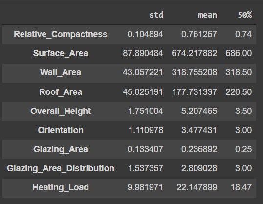

Building and Evaluating An Initial Model Using The Original Data

We will be using the Catboost algorithm to build our model. We won't be fine-tuning the parameters to avoid distorting the influence of imputations later on. We will also be evaluating the Mean Absolute Error of our predictive model.

# import required packages
from catboost import CatBoostRegressor
from sklearn.metrics import mean_absolute_error

# get the features and targets
# for train and test sets
x_train = train_df.drop('Heating_Load', axis=1)
y_train = train_df['Heating_Load']
x_test = test_df.drop('Heating_Load', axis=1)
y_test = test_df['Heating_Load']

# Build and train the model 
model = CatBoostRegressor()
model.fit(x_train, y_train)

# Evaluate the model on test set
original_score = mean_absolute_error(y_test, model.predict(x_test))
print(f'The MAE of the model using the original data is {original_score:.2f}') 

Simulating a Missing At Random Dataset

Now that we know what the performance of a model would look like using our original data, we can then simulate a Missing At Random dataset using our original dataset. We will be using sample codes from this paper to generate a Missing at Random absence in the original data.  You can check out the full code on the paper's repo.

# import required packages
import torch
import wget
wget.download('https://raw.githubusercontent.com/BorisMuzellec/MissingDataOT/master/utils.py')
from utils import *

# Function produce_NA for generating missing values

def produce_NA(X, p_miss, mecha="MAR", opt=None, p_obs=None, q=None):
    
    to_torch = torch.is_tensor(X)
    
    if not to_torch:
        X = X.astype(np.float32)
        X = torch.from_numpy(X)
    
    if mecha == "MAR":
        mask = MAR_mask(X, p_miss, p_obs).double()
    elif mecha == "MNAR" and opt == "logistic":
        mask = MNAR_mask_logistic(X, p_miss, p_obs).double()
    elif mecha == "MNAR" and opt == "quantile":
        mask = MNAR_mask_quantiles(X, p_miss, q, 1-p_obs).double()
    elif mecha == "MNAR" and opt == "selfmasked":
        mask = MNAR_self_mask_logistic(X, p_miss).double()
    else:
        mask = (torch.rand(X.shape) < p_miss).double()
    
    X_nas = X.clone()
    X_nas[mask.bool()] = np.nan
    
    return X_nas.double()

Now let's create our MAR dataset using the function.

# get sample MAR data 
data_MAR = produce_NA(train_data.to_numpy(), p_miss=0.20, p_obs=0.75)

# load MAR data into dataframe
MAR_df = pd.DataFrame(data_MAR.numpy(), columns= train_data.columns)
MAR_df.sample(5)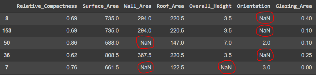

Now we have our dataset with MAR absence. Before applying the techniques to handle absence in our data, let's evaluate the extent of absence in the data and check the affected variables.

# Total Percentage of missing values
total_miss_percent = (sum(MAR_df.isnull().sum()) / (MAR_df.shape[0] *                                                             MAR_df.shape[1])) * 100
print(f'Percentage of total missing data: {total_miss_percent:.0f}%')

7% of our data is missing. This seems quite minimal. Here, we should consider deleting the missing values as we would still have 93% of our data to work with. Let's see the distribution of absence in the data.

percent_missing = MAR_df.isnull().sum() * 100 / len(MAR_df)
pd.DataFrame(percent_missing, columns = ['Percent_Missing'])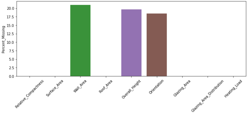

This shows that only 3 features are affected by missing values with a maximum of 20% absence. It is thus inappropriate to drop the features with missing values. Let's go a step further and check the number of  samples affected by absence.

Percent_miss_samples = ((len(MAR_df) - len(MAR_df.dropna())) / len(MAR_df)) *  100 
print(f'Percentage of samples with missing data: {Percent_miss_samples:.0f}%')

The location of missing values in the data is such that we will be throwing away 48% of the samples in our data with listwise deletion. This is quite a considerable amount of data that is inappropriate to delete.

In real-life situations, we will also need to understand the mechanism behind the absence. Even though we know we have generated a MAR scenario, we will not know this beforehand. This would require some missing data analysis on our data. T-tests and chi-square tests between variables are helpful in determining the relative relationships between variables in the data. The Missingno package also contains efficient tools to easily visualize the relationships of absence among variables.

APPLYING TECHNIQUES FOR HANDLING MISSING DATA

Several methods are employed for handling absence in datasets. These range from simple imputations to complex algorithms. These techniques are not without pros and cons, with modern techniques often edging out on efficiency. Certain techniques are often more appropriate for specific absence and extent of the missing data. A summary of these methods is shown below.

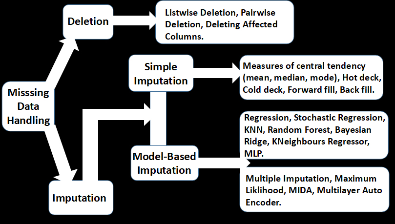
Deletion

Deletion involves removing missing values from the dataset. This includes listwise, pairwise, and featurewise deletions. In listwise deletion, all samples affected by absence are removed at once from the dataset.  In pairwise deletion, samples with missing observations are excluded for particular analysis where such observations are not needed, but included in other analysis for which their available observations are required. This is the method employed for correlation analysis.

Featurewise deletion is less popular and particularly inefficient as it involves removing features with missing data. This is only useful when the features are much less important or hold very little available data. Either way,  practitioners often prefer listwise deletion removing missing values.

Let's apply listwise deletion to our MAR dataset.

# drop sample with missing values
listwise_df = MAR_df.dropna()

# get data description after deletion
listwise_desc = listwise_df.describe().T[['std', 'mean', '50%' ]]

print(f'Number of samples before deletion: {len(MAR_df)}')
print(f'Number of samples after deletion: {len(listwise_df)}')
print(f'Number of samples after lost to listwise deletion: {len(MAR_df) - len(listwise_df)}')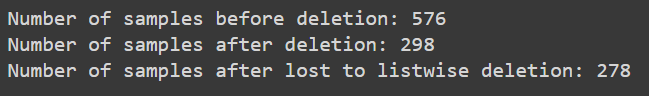

As we saw earlier, we are losing a considerable amount of data to deletion.  Let's see how that affects the performance of our model.

# Get the features and target variables
# of the dataset after listwise deletion
x_train = listwise_df.drop('Heating_Load', axis=1)
y_train = listwise_df['Heating_Load']

# building and evaluating the model
model = CatBoostRegressor()
model.fit(x_train, y_train)
listwise_score = mean_absolute_error(y_test, model.predict(x_test))
print(f'The MAE of the model using listwise deletion is {listwise_score :.2f}')

The performance is worse than with the complete data. This is as expected because:

I. The absence in our case is quite significant (about 50% of the data). Using listwise deletion reduces the sample size and distribution considerably. This consequently reduces the performance of the model as the sample size becomes inadequate to properly model the variance and correlations in the data.

II. Vital information for modelling the relationships specific to those missing samples is lost. This is particularly problematic for MAR cases, as such relationships are important since the absent data is correlated to the observed variables. Therefore, listwise deletion produces biased parameters and estimates in this scenario.

Imputation

Missing data imputation involves replacing the missing data with substituted values. There are different approaches to imputing values for values data.

1. Simple Imputation: This is the easiest form of imputation. It generally involves replacing missing values in a variable with an aggregate measure or interpolation of non-missing values in the variable. The observations in other variables are not used to infer the missing values in the affected variable. Certain measures of central tendency (mean, median, mode) are commonly used to simply substitute the missing values in the variable.                                     Other simple techniques include the Hot Deck imputation, where a missing value is replaced with an observed response from a similar unit; as opposed to the Cold deck imputation where dissimilar units are used. Forward and backwards fill imputations involves filling missing values with the preceding or successive values in the variable. They are commonly used for handling time-series data.

We will be applying the most commonly used mean and median imputations for our comparison. Scikit-Learn's Simple Imputer provides convenient methods for simple imputation.

# import required package
from sklearn.impute import SimpleImputer

# define mean imputer
imputer = SimpleImputer(missing_values=np.nan, strategy='mean')

# get mean of variables and substitute missing values
mean_imp_data = imputer.fit_transform(MAR_df.values)

# get dataframe with mean imputed values
mean_imp_df = pd.DataFrame(mean_imp_data, columns= MAR_df.columns)

# get data description after mean imputation
mean_imp_desc = mean_imp_df.describe().T[['std', 'mean', '50%' ]]

We have substituted all missing values in each variable with the mean of the respective variable. We can now check the performance of our model using our mean imputed dataset.

# get the train features and target variables
# of the mean imputed dataset
x_train = mean_imp_df.drop('Heating_Load', axis=1)
y_train = mean_imp_df['Heating_Load']

# building and evaluating the model
model = CatBoostRegressor()
model.fit(x_train, y_train)
mean_imp_score = mean_absolute_error(y_test, model.predict(x_test))
print(f'The MAE of the model using mean imputation is {mean_imp_score :.2f}')

Despite using twice as much data as with listwise deletion, we get similar performance. We could follow the same steps for median imputation by simply changing the 'mean' strategy for the imputer to 'median' to get the result below.

Using median imputation performs better than using mean imputation, but still worse than with the original data. This could happen because:

I. Simple imputation does not reflect the dispersion or variance in the data. The variance of the imputed values will be zero which would most probably not be the case in real life. This produces biased estimates of the variance and covariance as the dispersion is incorrectly modelled.

II. Simple Imputation leads to underestimated standard errors. This is because the imputations are only estimates of the original values, but are treated as exact data by the predictive algorithms. The errors between the real and estimated values are underestimated, making the model biased.

III. Depending on the type of distribution, the median is often a more robust measure of central tendency. This is usually because the mean is easily distorted by outliers and asymmetric distributions.              

2. Model-Based Imputation: Model-based imputations utilize statistical algorithms for estimating missing values. This usually involves using the available data from other variables in estimating the missing values for each variable in the dataset. Commonly used models include Stochastic Regression, Random Forest, KNN, Bayesian Ridge and K Neighbours Regressor.

We will be using the K Neighbours Regressor for our model-based imputation. This choice, with Random Forest, is usually preferable as it does not need much hypertuning and easily handles non-linear relationships in data. While the algorithms should be tuned for more efficiency in real life, we will use the default values so as not to influence the model's performance. Scikit-Learn's Iterative Imputer provides convenient methods for applying model-based Imputation multiple times on a single dataset.

# import required packages
from sklearn.experimental import enable_iterative_imputer
from sklearn.impute import IterativeImputer
from sklearn.neighbors import KNeighborsRegressor

# define model for imputation
impute_estimator = KNeighborsRegressor()
imputer = IterativeImputer(estimator=impute_estimator, max_iter=25, tol= 1e-1, random_state=0)

# impute missing values using model imputer
model_imp_data = np.round(imputer.fit_transform(MAR_df), 6)

# get datafraame with model imputation
model_imp_df = pd.DataFrame(model_imp_data, columns= MAR_df.columns)

# get description of model imputed data
model_imp_desc = model_imp_df.describe().T[['std', 'mean', '50%' ]]

After imputing for all missing values in the data using our imputer model. We can then check the performance of our estimator.

# get the train features and target variables
# of the model imputed dataset
x_train = model_imp_df.drop('Heating_Load', axis=1)
y_train = model_imp_df['Heating_Load']

# building and evaluating the model
model = CatBoostRegressor()
model.fit(x_train, y_train)
model_imp_score = mean_absolute_error(y_test,model.predict(x_test))
print(f'The MAE of the model using model based imputation is {model_imp_score :.2f}')

Without hypertuning our imputation model, we already get a better performance than the previous techniques. This is mostly because the algorithms utilize multiple variables to estimate the missing values, unlike simple imputations.

Modern Approaches

There are few modern approaches to handling missing data with more efficient statistical properties. The most common ones in literatures are FIML and Multiple Imputation

1. Full Information Maximum Likelihood (FIML): This method does not impute data, but rather uses available data to compute maximum likelihood estimates. Likelihood estimation is a method of estimating the parameters of an assumed probability distribution given some observed data.  Maximizing the likelihood function for such estimations is known as Maximum Likelihood Estimation. When data is missing, we can factor the likelihood function which is computed separately for cases with complete data on some variables and those with complete data on all variables. These two likelihoods are then maximized together to find the estimates.This method is however limited to linear models and there are no standard Maximum Likelihood Imputations for diverse distributions.
2. Multiple Imputation: This is an extension of the model-based imputation but involves numerous iterations of imputations to model the variance well enough to correct the standard errors that arise from model imputation. As earlier stated, model-based imputation does not account for the standard prediction errors that arise from estimating the missing values, which leads to the inefficiency of the predictive model. Multiple Imputation addresses this problem by carrying out Model-based Imputation several times over, creating numerous replicas with slightly different imputations, such that the predicted missing values become roughly as distributed as the population of the original values. Because of the variation in the imputed values, there would be variation in the parameter estimates, leading to appropriate estimates of standard errors.

The workflow of the Multiple  Imputation technique generally includes:

1. Introduce random variations into the process of imputing missing values
2. Generate several datasets with slightly different imputed values
3. Perform predictive analysis on each of the datasets
4. Combine the results into a single set of parameter estimates by mean aggregation

We will be using the MiceForest package, which utilizes LightGBM algorithm to implement MICE, a type of Multiple Imputation technique that uses Chained Equations to run multiple modelling for each missing value conditionally, using the observed values, to replace the missing values in our dataset.

# import required package
import miceforest as mf

# create kernel for MI
kernel = mf.ImputationKernel(MAR_df, datasets=20, random_state= 0)

# Run the MICE algorithm for 5 iterations
#  on each of the datasets
kernel.mice(5)

# show the number of datasets
print(f'Number of datasets with imputations: {kernel.dataset_count()}')

We now have multiple datasets with different imputations, the next step is to aggregate our datasets for predictive modelling, there are three ways main ways to do this:

1. Get the mean aggregates of the datasets as a single dataset and use it to build our predictive model.
2. Build multiple models with our datasets and use the mean aggregate of the models' parameters to create a single predictive function.
3. Build multiple models with our datasets and use the mean aggregate of their predictions as final prediction.

Options 2 and 3 are often better choices. This is because in option 1, the imputations with more variance will tend towards the mean, and the variance of overall imputations will be lowered, resulting in a final dataset which does not model the dispersion in the original dataset.

# For each imputed dataset, train a catbost regressor
predictions = []
for i in range(kernel.dataset_count()):
    MICE_imp_df = kernel.complete_data(i)
    x_train = MICE_imp_df.drop('Heating_Load', axis=1)
    y_train = MICE_imp_df['Heating_Load']
    model = CatBoostRegressor()
    model.fit(x_train, y_train)
    predictions.append(model.predict(x_test)) # add test prediction to list
    
# get mean of predictions and evaluate on test set    
mean_predictions = (np.array(predictions)).mean(axis=0) 
MICE_imp_score = mean_absolute_error(y_test, mean_predictions)
print(f'The MAE of the model using multiple imputation is {MICE_imp_score :.2f}')

With only 20 datasets we match the performance of our model-based approach (which performed really well for this problem). Most literature recommends between 20 to 100 datasets, depending on the number of missing values and available computing resources (as multiple imputations can be resource intensive). You can always experiment with a higher number of imputations and compare their performances on specific datasets.

Summary:

We examined different missing data imputation techniques and compared their performances on building predictive models with data that has MAR data absence. We mainly implemented listwise deletion, simple imputation with mean and median strategies, model-based- imputation with K Nearest Regressor and a modern imputation approach using multiple imputation.

Deletion loses vital information for efficient modelling and are generally a bad idea. They should only be used when the absence is negligible and the sample size is adequate enough to model the relationships in the data.

Mean imputation is no better as it doesn't model the variance of the missing values and is biased for asymmetrical distributions, for which midian imputation is often a better choice. While simple imputation methods are generally deemed appropriate for specific absence, such as normally distributed and MCAR absence, they are problematic when modeling MAR and MNAR absence.      

Model-based approaches utilize multivariate modeling using statistical algorithms to address the faults of simple imputations to improve performance. While they improve  on simple imputations, they also do not account for the standard errors in predicting missing values.

Finally, we looked at modern approaches such as Multiple Imputation and Full maximum Likelihood. We implemented Multiple Imputation using MICE whose performance matched the result of the Model-based approach with only 20 datasets. Mordern approaches are generally more efficient as they more appropriately estimates the standard errors.

While this is not an exhaustive list of handling techniques and we could also carry out deeper comparisons of the statistical properties of the generated datasets, I hope this give insights into the faults of most commonly used techniques and shows how modern approaches address these faults in improving the effectiveness of missing data handling.