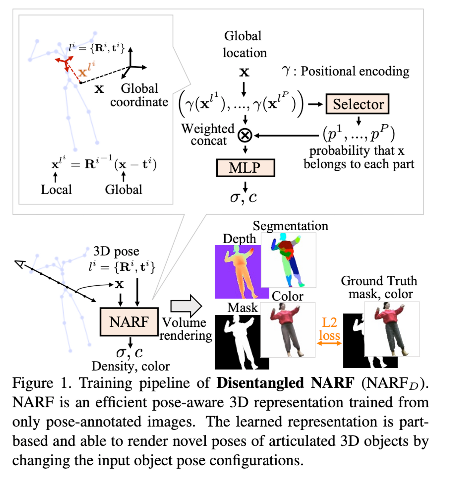
The goal of this project is to learn the pose-controllable representations of articulated objects. To achieve this they consider the rigid transformation of the most relevant object part in solving dot the radiance field at each location.

Inverse Graphics Paradigm: This is when you analyze an image by attempting to synthesize it with compact graphics codes. Modeling articulated 3D objects using neural nets remains challenging due to the large variance of joint locations, self-occlusions, and high non-linearity in forward kinematic transformations.
They extend the NeRF architecture to represent 3D articulated objects (NARF). This is challenging because of a couple of reasons:
- There exists a non-linear relationship that exists between a kinematic representation of 3D articulations and the resulting radiance field making it difficult to model implicitly in a neural network.
- The radiance field at a given 3D location is influenced by at most a single articulated part and its parents along the kinematic tree, while the full kinematic model is provided as input. This may result in the model learning dependencies of the output to the irrelevant parts which limits the generalization of the model.
Their solution to these challenges include:
- A method to predict the radiance field at a 3D location based on only the most relevant articulated part that is identified using a set of sub-networks that output probability for each given part given the 3D location and geometric configuration of the parts.
- The spatial configurations of parts are computed explicitly with a kinematic model as opposed to implicitly in the network.
- A NARF then predicts the density and view-dependent radiance of the 3D location conditioned on the properties of only the selected part.
NARF METHOD
Pose-Conditioned NeRF: A Baseline
- The radiance of a 3D location is thus conditioned on the pose configuration. Once the pose-conditioned NeRF is learned, novel poses can be rendered in addition to novel views by changing the input pose configurations.
The Kinematic Model
This model represents an articulated object of P+1 joints, including end-points, and P bones in a tree structure where one of the joints is selected as the root joint and each remaining joint is linked to its single parent joint by a bone of fixed length.
The root joint is defined by a global transformation matrix $T^0$
$ζi$
is the bone length from the $i^{th}$ joint $J_i$ to its parent, $i \\in \\{1,...P\\}$, and $\\theta_i$ denotes the rotation angles of the joint w.r.t its parent joint.
A bone defines a local rigid transformation between a joint and its parent, therefore the transformation matrix $T_{local}^i$ is computed as:
$T_{local}^i = Rot(ζi)$, where Rot and Trans are the rotation and translation matrices respectively.
The global transformation from the root joint to join $J_i$ can thus be obtained by multiplying the transformation matrices along the bones from the root to the $i^{th}$ joint:
$T^i = (Π_{k∈Pa(i)}T^k_{local})T^0$
where $Pa(i)$ includes the $i^{th}$ joint and all its parent joints along the kinematic tree.
The corresponding global rigid transformation $l^i ={R^i,t^i}$ for the $i^{th}$ joint can then be obtained from the transformation matrix $T^i$.
To condition the radiance field at 3D location $x$ on a kinematic pose configuration $P = \{ T^0, ζ, \theta \}$
they concatenate a vector representing $P$ as the model input.
The Conditioned New Model
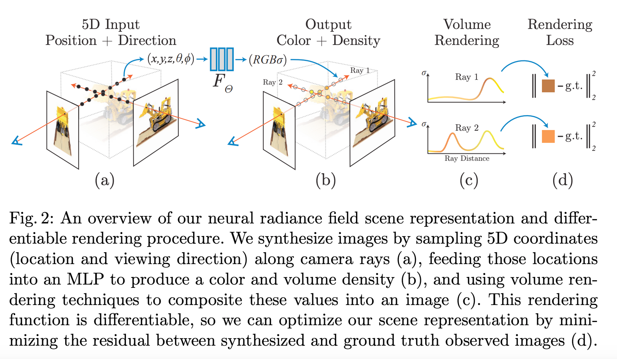
We know that the standard NeRF takes in the 3D point and the viewing direction and outputs the density and color of that point as predicted by an MLP [Mildenhall, Ben, et al.] NeRFs take in a 5D vector input for each point on the pixel/ray: the position coordinates $(x,y,z)$ and the viewing and rotation angles $(\theta, \phi)$ → $[x,y,z,\theta, \phi]$ and they output a 4D vector representing the output color $(RGB)$ and density $(\sigma)$ of that point → $[R,G,B,\sigma]$

In NARF, the neural radiance field model is conditioned on the kinematic pose configuration to give a new model:
$[x,y,z, \{l_i|i=1,...,P\},\theta, \phi \rightarrow [\sigma, c]$
What are the building blocks of this function?
To begin, they estimate the radiance field in the object coordinate system where the density is constant w.r.t a local 3D location. This estimation takes the form:
$F: (x^l) \rightarrow (\sigma, h)$
To condition the model on shape variation, we condition the model on bone parameter $ζ$, to create a new function that takes the form:
$F: ((x^l),(ζ)) \rightarrow (\sigma, h)$
The color at a 3D location is dependent on changes in the lighting from a viewing direction $d$ and the rigid transformation $l$. So, they use a 6D vector representation
				$ξ$


	of transformation $l$ as the network input. To factor in the viewing direction and vector representation of the transformation, they get a new function of the form:
$F_{\theta_c}^{l,ζ} : (h, (d^l), ξ) \rightarrow c$ while $d^l = R^{-1}d$
**** I think $h$ is a location/region/3D coordinate that has consistent desnity → I’ll have to re-read the paper to be sure.
The final model function that combines all of these building blocks is:
$F_\theta^{l,ζ} = (x^l, d^l, ξ, ζ) \rightarrow (c,\sigma)$
They train 3 different NARF models to explore various architectures that would efficiently actualize the model function.
Part-Wise NARF $(NARF_p)$
In this architecture, they train a separate NARF for each part in the articulated body and then merge the outputs to get the global representation of the entire body. Given the kinematic 3D pose configuration $\{T^0, ζ, \theta\}$ of an articulated object, compute the global rigid transformation $\{l_i|i=1,...,P\}$ for each rigid part using forward kinematics.
To estimate the density and color $(\sigma, c)$ of a global 3D location $x$ from a 3D viewing direction $d$, we train a separate RT-NeRF for each part $x^{l^i}$ where
$x^{l^i} = R^{i^{-1}}(x-t^i), d^i = R^{i^{-1}}d$ and the NARF for each part is computed from this formula:
$F: (x^{l^i}, d^{l^i},ξ^i, ζ) \rightarrow (c^i, \sigma^i)$
They combine the densities and colors estimated by the different RT-NeRFs into one. The density and color of a global 3D location $x$ can be determined by taking the estimate with the highest density as determined by applying a softmax function. Finally, they use volume rendering techniques on the selected color and density values to render the 3D object.
The rendering and softmax operations are differentiable therefore image reconstruction loss can be used to update the gradients. $NARF_p$ is computationally inefficient because a model is optimized for each part. Because of the need to apply a softmax function to all the predicted color and density values per part, training is dominated by a large number of zero-density samples.
Holistic NARF ($NARF_H)$
This method combines the input s of the RT-Nerf models in $NARF_p$ and then feeds them as a whole into a single NeRF model for direct regression of the final density and color $(\sigma, c)$
$F_\theta : Cat(\{(x^l)|i \in [1,...,P]\},(ξ)) \rightarrow (\sigma, h)$
$F_{\theta} : Cat(h,\{((d^{l^i}), (ζ^i))| i \in [1,...,P]\} \rightarrow (c)$
$Cat:$ is the concatenation operator
The advantage of this new architecture is that there is only a single NARF trained, and the computational cost is almost constant to the number of object parts. The disadvantage of $NARF_H$ does not satisfy part dependency because all parameters are considered for each 3D location. This means that object part segmentation masks cannot be generated without dependencies.
Disentangled NARF $(NARF_D)$
While considering the merits and demerits of $NARF_p$ and $NARF_H$ , the authors introduce a selector, $S$, which identifies which object part a global 3D location $x$ belongs to. $S$ consists of $P$ lightweight subnetworks for each part. A subnetwork takes in the local 3D position of $x$ in $l^i = \{R^i, t^i\}$ and the bone parameter as inputs and outputs the probability $p^i$ of $x$ belonging to the $i^{th}$ part. The softmax function is then used to normalize the selector's outputs.
For implementation, they use a two-layer MLP with ten nodes for each occupancy network which is a lightweight and effective solution. $NARF_D$ softly masks out irrelevant parts by masking their inputs. The resulting input is still in the form of a concatenation.
The result is in the form of a concatenation because all bones share the same NeRF which needs to distinguish them to output the correct density $\sigma$ and color $c$. The selector outputs probabilities of a global 3D location belonging to each part and then generated a segmentation mask by selecting the locations occupies by a specific part.
Summary
NARF is a NeRF conditioned on kinematic information that represents the spatial configuration of a 3D articulated object. The 3 different NARFs described above take in the 5D input vector describing the 3D location and viewing direction and output the radiance field based on the most relevant articulated part. Using NARF it is possible to get a more realistic and semantically correct 3D representation of 3D articulated objects that can be used as artifacts for video editing, filmmaking, and video game production.
Citations:
Noguchi, Atsuhiro, et al. "Neural articulated radiance field." Proceedings of the IEEE/CVF International Conference on Computer Vision. 2021.
Mildenhall, Ben, et al. "Nerf: Representing scenes as neural radiance fields for view synthesis." Communications of the ACM 65.1 (2021): 99-106.


