In the first two parts of our series on NumPy optimization, we have primarily covered how to speed up your code by trying to substitute loops for vectorized code. We covered the basics of vectorization and broadcasting, and then used them to optimize an implementation of the K-Means algorithm, speeding it up by 70x compared to the loop-based implementation.
Following the format of Parts 1 and 2, Part 3 (this one) will focus on introducing a bunch of NumPy features with some theory–namely NumPy internals, strides, reshape and transpose. Part 4 will cover the application of these tools to a practical problem.
In the earlier posts we covered how to deal with loops. In this post we will focus on yet another bottleneck that can often slow down NumPy code: unnecessary copying and memory allocation. The ability to minimize both issues not only speeds up the code, but may also reduce the memory a program takes up.
We will begin with some basic mistakes that can lead to unnecessary copying of data and memory allocation. Then we'll take a deep dive into how NumPy internally stores its arrays, how operations like reshape and transpose are performed, and detail a visualization method to compute the results of such operations without typing a single line of code.
In Part 4, we'll use the things we've learned in this part to optimize the output pipeline of an object detector. But let's leave that for later.
Before we begin, here are the links to the earlier parts of this series.
 Ayoosh Kathuria
 Ayoosh Kathuria
Bring this project to life
So, let's get started.
Preallocate Preallocate Preallocate!
A mistake that I made myself in the early days of moving to NumPy, and also something that I see many people make, is to use the loop-and-append paradigm. So, what exactly do I mean by this?
Consider the following piece of code. It adds an element to a list during each iteration of the loop.
li = []
import random


for i in range(10000):
	# Something important goes here
    x = random.randint(1,10)
    li.append(x)
The script above merely creates a list containing random integers from zero to nine. However, instead of a random number, the thing we are adding to the list could be the result of some involved operation happening every iteration of the loop.
append is an amortized O(1) operation in Python. In simple words, on average, and regardless of how large your list is, append will take a constant amount of time. This is the reason you'll often spot this method being used to add to lists in Python. Heck, this method is so popular that you will even find it deployed in production-grade code. I call this the loop-and-append paradigm. While it works well in Python, the same can't be said for NumPy.
When people switch to NumPy and they have to do something similar, this is what they sometimes do.
# Do the operation for first step, as you can't concatenate an empty array later
arr = np.random.randn(1,10)

# Loop
for i in range(10000 - 1):
        arr = np.concatenate((arr, np.random.rand(1,10)))
Alternatively, you could also use the np.append operation in place of np.concatenate. In fact, np.append internally uses np.concatenate, so its performance is upper-bounded by the performance of np.concatenate.
Nevertheless, this is not really a good way to go about such operations. Because np.concatenate, unlike append, is not a constant-time function. In fact, it is a linear-time function as it includes creating a new array in memory, and then copying the contents of the two arrays to be concatenated to the newly allocated memory.
But why can't NumPy implement a constant time concatenate, along the lines of how append works? The answer to this lies in how lists and NumPy arrays are stored.
The Difference Between How Lists And Arrays Are Stored
A Python list is made up references that point to objects. While the references are stored in a contiguous manner, the objects they point to can be anywhere in the memory.
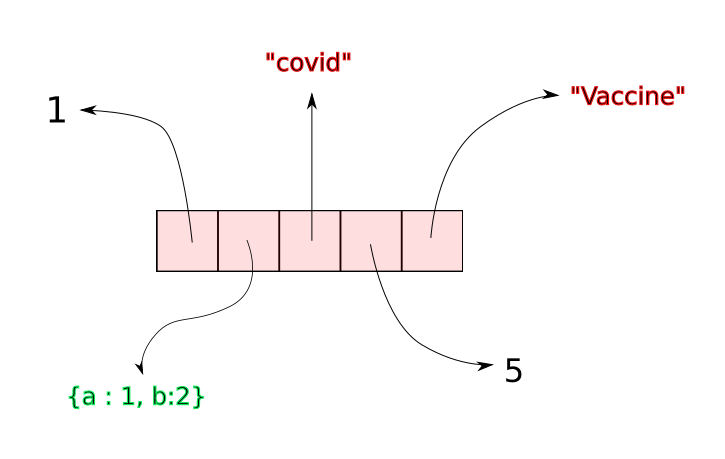
Whenever we create a Python List, a certain amount of contiguous space is allocated for the references that make up the list. Suppose a list has n elements. When we call append on a list, python simply inserts a reference to the object (being appended) at the $ {n + 1}^{th} $ slot in contiguous space.
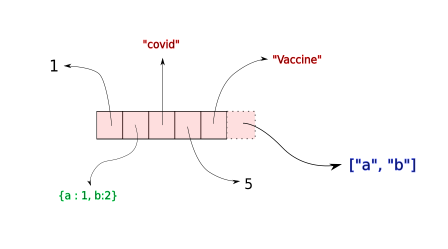
Once this contiguous space fills up, a new, larger memory block is allocated to the list, with space for new insertions. The elements of the list are copied to the new memory location. While the time for copying elements to the new location is not constant (it would increase with size of the array), copying operations are often very rare. Therefore, on an average, append takes constant time independent of the size of the array
However, when it comes to NumPy, arrays are basically stored as contiguous blocks of objects that make up the array. Unlike Python lists, where we merely have references, actual objects are stored in NumPy arrays.
All the space for a NumPy array is allocated before hand once the the array is initialised.
a = np.zeros((10,20)) # allocate space for 10 x 20 floatsThere is no dynamic resizing going on the way it happens for Python lists. When you call np.concatenate on two arrays, a completely new array is allocated, and the data of the two arrays is copied over to the new memory location. This makes np.concatenate slower than append even if it's being executed in C.
To circumvent this issue, you should preallocate the memory for arrays whenever you can. Preallocate the array before the body of the loop and simply use slicing to set the values of the array during the loop. Below is such a variant of the above code.
arr = np.zeros((10000,10))

for i in range(10000):
    arr[i] = np.random.rand(1,10)
Here, we allocate the memory only once. The only copying involved is copying random numbers to the allocated space and not moving around array in memory every iteration.
Timing the code
In order to see the speed benefits of preallocating arrays, we time the two snippets using timeit.
%%timeit -n 100

arr = np.random.randn(1,10)
for i in range(10000 - 1):
        arr = np.concatenate((arr, np.random.rand(1,10)))
The output is

Whereas for the code with pre-allocation.
%%timeit -n 10

arr = np.zeros((10000,10))

for i in range(10000):
    arr[i] = np.random.rand(1,10)
We get a speed up of about 25x.

Views and Copies
Here's another seemingly innocuous mistake than can actually slow down your code. Consider that you have to slice an array with continuous indices.
a = np.arange(100)

sliced_a = a[10:20]
However, you could have achieved the same with the following snippet of code.
a = np.arange(100)

sliced_a = a[range(10,20)]
This is called Fancy Indexing where you pass a list or a tuple as index instead of plain old slicing. It is useful when we want to get a list made up of indices which are non-continuous like getting the the $ 2^{nd}$ , $7^{th}$ and $11^{th} $ indices of an array by doing arr[[2,7,11]].
However, do you think both are the same in terms of computation speed. Lets time them up.
a = np.arange(100)

%timeit -n 10000 a[10:20]
%timeit -n 10000 a[range(10,20)]
Here is my output.

We see running times of a different order! The normal slicing version takes about 229 nanoseconds while the fancy-indexing take about 4.81 microseconds which is 4810 nanoseconds, i.e fancy-indexing is slower by around 20 times!
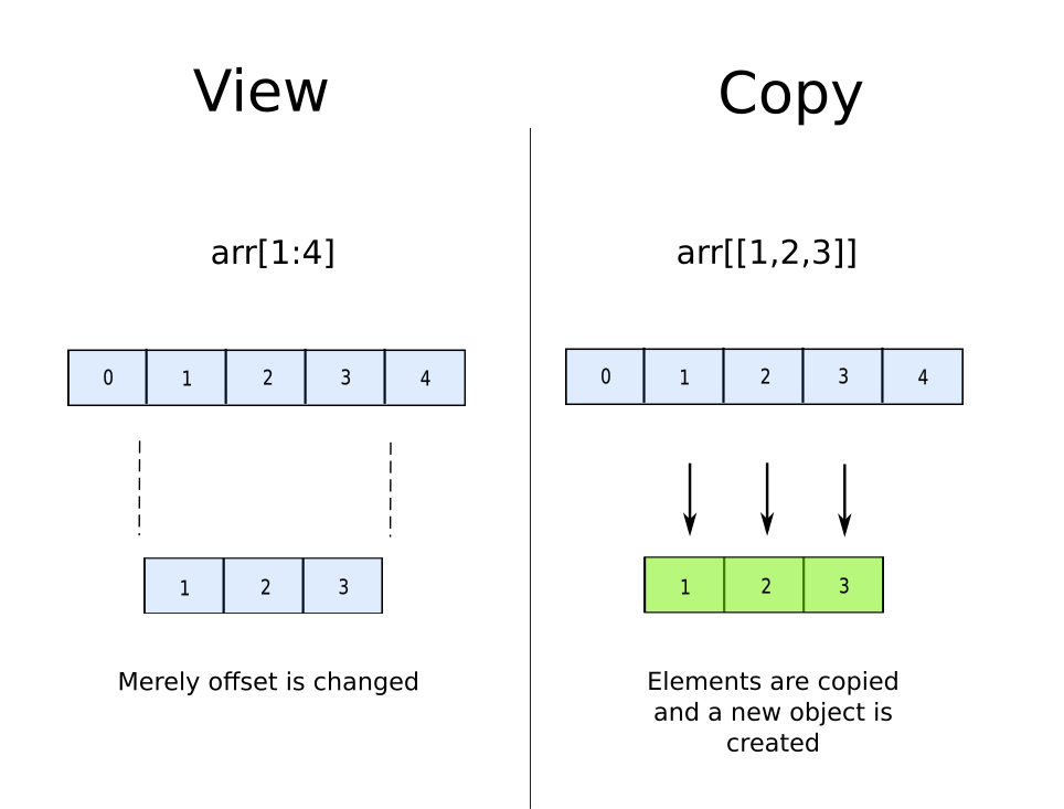
This happens because normal slicing has to merely return a new offset. You do not need to create a copy of the data as the sequence of the data in the slice remains the same as the original array, and therefore you could simply change the starting point of the array.
However, when one goes for fancy-Indexing, a copy is created. Why? Because NumPy array are implemented as contiguous blocks in memory. When we index something like a[[2,7,11]], the objects at the indices 2, 7 and 11 are stored in a non-contiguous manner. You can not have the elements of the new array lined up in a contiguous manner unless you make a copy.
The take away lesson here would be if you have continuous indices to slice, always chose normal slicing over fancy indexing.
In the next section, we will gloss over how internals of NumPy, how arrays are stored, what happens under the hood when we reshape or transpose operations.
NumPy internals
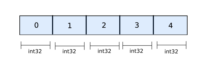
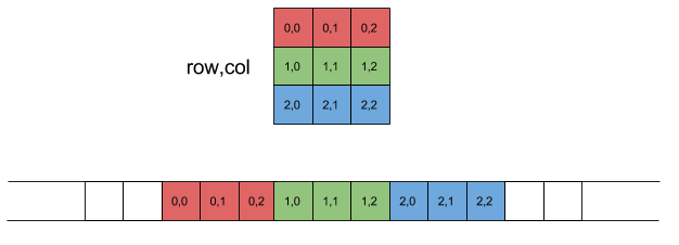
In NumPy, regardless of the shape of the array, internally arrays are stored as contiguous block of objects. However, what helps us work with them as if they are multi-dimensional arrays is something called strides.
For example consider the follow array.
[[ 0  1  2  3]
 [ 4  5  6  7]
 [ 8  9 10 11]]
This array is basically stored in the memory as follows.
[ 0 1 2 3 4 5 6 7 8 9 10 11]
In order to emulate dimensions for a contiguous block of objects, NumPy uses strides. We have a stride for each dimension. For example, for the array above, the strides would be (32, 8). But what do strides actually mean?
It means that if you want to go to the index [1,3] for the 2-D array, you will have to go to the memory location that is 1 * 32 + 3 * 8 or 56 bytes from the starting. Each integer takes up 32 bits or 8 bytes of memory. This means 56 bytes from the starting corresponds to 7 integers. Therefore, when we query index [1,3] we get the integer after 7 integers, i.e. index number 8, which has the value 7.
print(arr[1,3])
# Output -> 7
In other words, stride for a dimension basically tells you how much blocks of physical memory you must skip in the contiguous memory to reach the next element in that dimension while keeping the others constant. For e.g. consider index [0][2]. In order to jump to next element in the first dimension [1][2] , we must jump 32 bits in memory. Similarly, we jump 8 bits in physical memory to get to index [0][3].
Reshaping
The fact that NumPy stores arrays internally as contiguous arrays allows us to reshape the dimensions of a NumPy array merely by modifying it's strides. For example, if we take the array that we had above, and reshape it to [6, 2], the strides will change to [16,8], while the internal contiguous block of memory would remain unchanged.
a = np.arange(12).reshape(3,4)
print(a)

# Output
[[ 0  1  2  3]
 [ 4  5  6  7]
 [ 8  9 10 11]]

b = a.reshape(6,2)
print(b)

#Output
[[ 0  1]
 [ 2  3]
 [ 4  5]
 [ 6  7]
 [ 8  9]
 [10 11]]
We can also create dimensions. For example, we can reshape the original array to [2, 2, 3] as well. Here strides change to [48, 24, 8].
c = a.reshape(2,2,3)
print(c)

#Output
[[[ 0  1  2]
  [ 3  4  5]]

 [[ 6  7  8]
  [ 9 10 11]]]
Taking advantage of the way NumPy stores it's arrays, we can reshape NumPy arrays without incurring any significant computational cost as it merely involves changing strides for the array. The array, which is stored in a contiguous manner in the memory, does not change. Therefore, no copying is needed for reshaping.
In order to leverage this feature well, we must understand how reshaping works. Given an array and a target shape, we must be able to figure out what the reshaped array will look like. This will guide us in thinking along a solution that can be arrived through one or more reshaping operations.
How does reshaping work?
We now dwell into how reshaping works. When trying to explain how shapes work in NumPy, a lot of people insist on imagining arrays as grids and cubes.
However, the moment you go beyond 3-D, visualisation becomes really problematic. While we can use cubes for 2-D and 3-D arrays, for higher dimensions we must come up with something else.
So what I propose instead, is to imagine the array like a tree. Each level of the tree represents a dimension in the original order. For example, the array that we covered above can be represented as follows.
[[ 0  1  2  3]
 [ 4  5  6  7]
 [ 8  9 10 11]]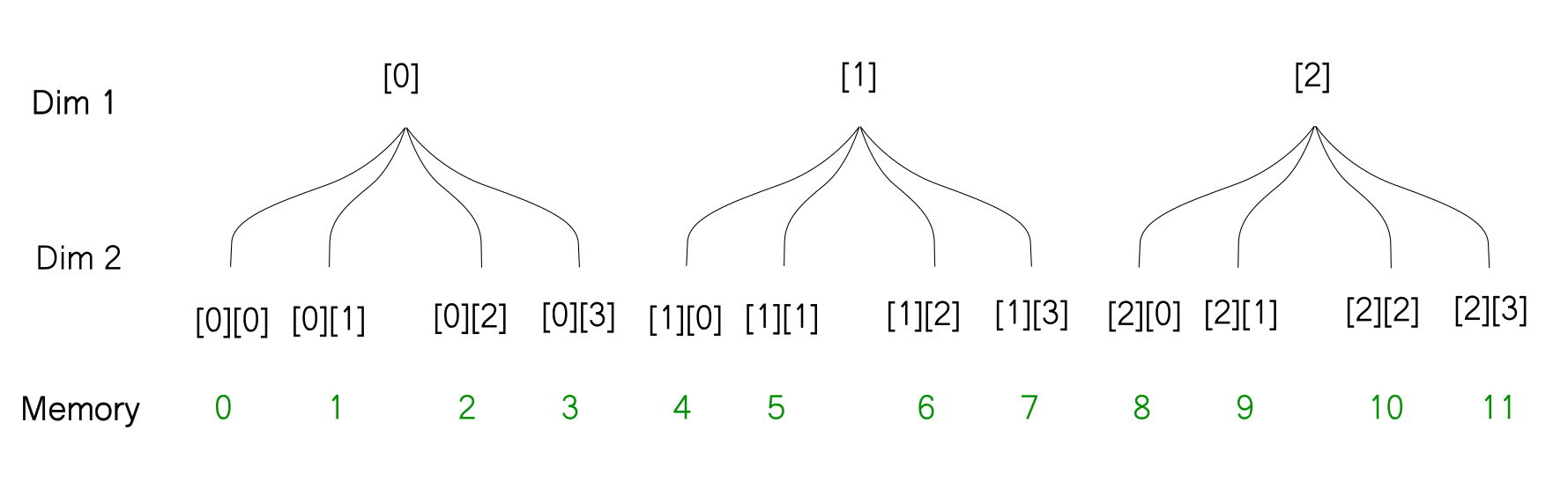
With this representation, it's very easy to figure out what will happen when you reshape an array. The thing to notice is that the reshaping does not change how the array is stored in memory. So when you reshape the array, the way the leaves of the tree are ordered does not change, only the way the branches are ordered changes. For example, when we reshape the above array from [3, 4] to [6,2] here is how we can imagine the reshaping operation using the tree diagram.
# Reshaped array -> [6, 2]

[[ 0  1]
 [ 2  3]
 [ 4  5]
 [ 6  7]
 [ 8  9]
 [10 11]]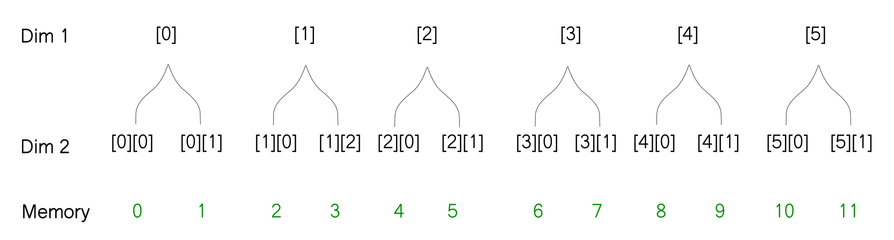
Here's an example where we reshape the array to [2, 2, 3].
[[[ 0  1  2]
  [ 3  4  5]]

 [[ 6  7  8]
  [ 9 10 11]]]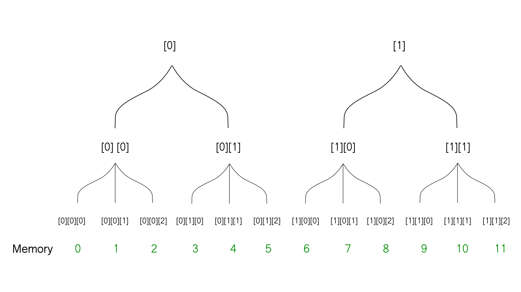
Transposing
Another operation that allows us to change the shape of arrays is the transpose function. It essentially enables us to swap dimensions of an array. We use the transpose operation for the same.
The argument to the transpose function is basically a mapping of indices from [0, 1, 2 .... n] to the new arrange of indices. For example, if I have an array of the shape [5 2 4], then using transpose(2, 0, 1) makes it [4 5 2] as the indices 0, 1, 2 are mapped to their new positions respectively.
c = a.transpose(1,0)

[[ 0  4  8]
 [ 1  5  9]
 [ 2  6 10]
 [ 3  7 11]]
The operation transpose itself does not require any copying because it merely involves swapping strides. While the strides for our original array were [32,8], for the transposed array they are [8, 32].
However, once we swap our strides, the array is no longer stored in what is called row-major format. Most of NumPy ops are designed to work on row-major arrays. Hence, there are many operations, (like flatten) , which when performed on a transposed array require a new array to be made. Explaining row-major and column-major is beyond the scope of this post. But here is a reference for curious souls.
When the new array is created, the order of the elements stored as a contiguous block changes. Consider the 2-D array which we transpose using mapping (0, 1). In the newly created array, an element corresponding to the index [a][b] is the swapped with element corresponding to the index [b][a] in the original array.
Returning to the tree visualisation, here is what the above transpose operation would look like.
The transposed array is of the shape [4,3]. We had earlier reshaped our original array to [4,3]. Notice that the two arrays are different, despite having the same shape. This is owing to the fact that the order of elements in the memory doesn't change for the reshape operation while it does change for the transpose operation.
Moving on to a more complicated example, let's consider a 3-D array where we swap more than one set of dimensions. It will be a bit complicated to show it using a tree-diagram so we are going to use code to demonstrate the concept. We use the transpose mapping (2, 0, 1) for a random array.
a = np.random.randint(100, size = (5, 7, 6))
b = a.transpose(2,0,1)
As above, any element that corresponds to the index [i][j][k] will be swapped with that corresponding the the index [k][i][j]. We can try this with the array above.
print(a[1,2,3] == b[3,1,2])
# output -> True

print(a[3,4,2] == b[2,3,4])
# output -> True
Conclusion
That's it for this post folks. In this post, we covered important topics like strides, reshaping and transpose. In order to build a command over these aspects of NumPy, I encourage you to think of examples similar to the ones in this post, and then tally the results with what you have learnt.
As promised in the beginning of the article, in the next part we will use a mixture of reshape and transpose operations to optimize the output pipeline of a deep learning based object detector. Till then, happy coding!
References