This is Part 4 of our ongoing series on NumPy optimization. In Parts 1 and 2 we covered the concepts of vectorization and broadcasting, and how they can be applied to optimize an implementation of the K-Means clustering algorithm. Next in the cue, Part 3 covered important concepts like strides, reshape, and transpose in NumPy. In this post, Part 4, we'll cover the application of those concepts to speed up a deep learning-based object detector: YOLO.
Here are the links to the earlier parts for your reference.
 Ayoosh Kathuria
 Ayoosh Kathuria
 Ayoosh Kathuria
Part 3 outlined how various operations like reshape and transpose can be used to avoid unnecessary memory allocation and data copying, thus speeding up our code. In this part, we will see it in action.
We will focus particularly on a specific element in the output pipeline of our object detector that involves re-arranging information in memory. Then we'll implement a naïve version where we perform this re-arranging of information by using a loop to copy the information to a new place. Following this we'll use reshape and transpose to optimize the operation so that we can do it without using the loop. This will lead to considerable speed up in the FPS of the detector.
So let's get started!
Bring this project to life
Understanding the problem statement
The problem that we are dealing with here arises due to, yet again, nested loops (no surprises there!). I encountered it when I was working on the output pipeline of a deep learning-based object detector called YOLO (You Only Look Once) a couple of years ago.
Now, I don't want to digress into the details of YOLO, so I will keep the problem statement very limited and succinct. I will describe enough so that you can follow along even if you have never even heard of object detection.
However, in case you are interested in following up, I have written a 5-part series on how to implement YOLO from scratch here.
Ayoosh Kathuria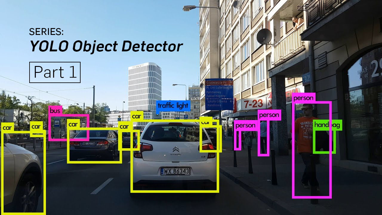
YOLO uses a convolutional neural network to predict objects in an image. The output of the detector is a convolutional feature map.
In case the couple of lines above sound like gibberish, here's a simplified version. YOLO is a neural network that will output a convolutional feature map, which is nothing but a fancy name for a data structure that is often used in computer vision (just like Linked Lists, dictionaries, etc.).
A convolutional feature map is essentially a spatial grid with multiple channels. Each channel contains information about a specific feature across all locations in the spatial grid. In a way, an image can also be defined as a convolutional feature map, with 3 channels describing intensities of red, green, and blue colors. A 3-D image, where each channel contains a specific feature.
Let's say we are trying to detect objects in an image containing a Rail engine. We give the image to the network and our output is something that looks like the diagram below.
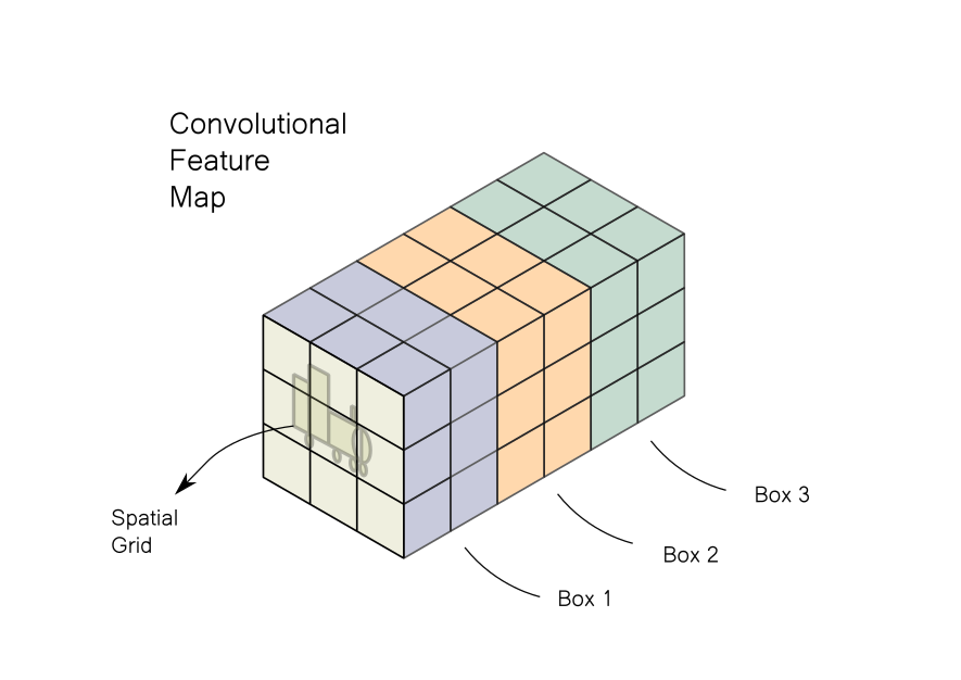
The image is divided into a grid. Each cell of the feature map looks for an object in a certain part of the image corresponding to each grid cell. Each cell contains data about 3 bounding boxes which are centered in the grid. If we have a grid of say 3 x 3, then we will have data of 3 x 3 x 3 = 27 such boxes. The output pipeline would filter these boxes to leave the few ones containing objects, while most of others would be rejected. The typical steps involved are:
- Thresholding boxes on the basis of some score.
- Removing all but one of the overlapping boxes that point to the same object.
- Transforming data to actual boxes that can be drawn on an image.
However, given the way information is stored in a convolutional feature map, performing the operations highlighted above can lead to messy code (for more details, refer to Part 4 of the YOLO series). To make the code easier to read and manage, we would like to take the information stored in a convolutional feature map and rearrange it to a tabular form, like the one below.
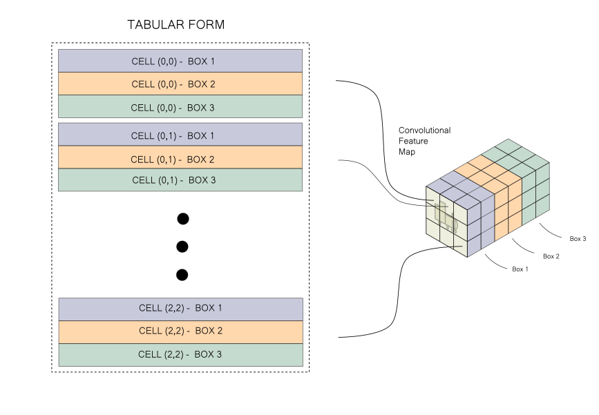
And that's the problem! We simply need to rearrange information. That's it. No need to go further into YOLO! So let's get to it.
Setting up the experiment
For the purposes of this experiment, I have provided the pickled convolutional feature map which can be downloaded from here.
We first load the feature map into our system using pickle.
import pickle
conv_map = pickle.load(open("conv_map.pkl", "rb"))
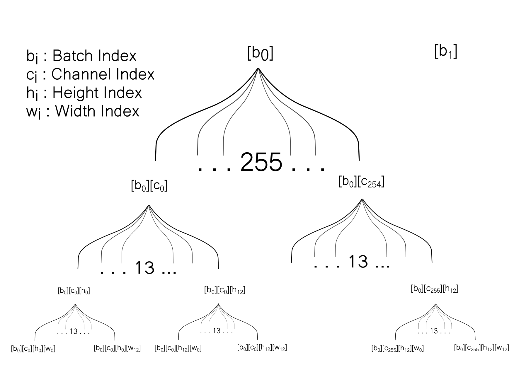
The convolutional neural network in PyTorch, one of most widely-used deep learning libraries, is stored in the [B x C x H x W] format where B is batch size, C is channel, and H and W are the dimensions. In the visualization used above, the convolutional map was demonstrated with format [H W C], however using the [C H W] format helps in optimizing computations under the hood.
The pickled file contains a NumPy array representing a convolutional feature map in the [B C H W] format. We begin by printing the shape of the loaded array.
print(conv_map.shape)
#output -> (1, 255, 13, 13)
Here the batch size is 1, the number of channels is 255, and the spatial dimensions are 13 x 13. 255 channels correspond to 3 boxes, with information for each box represented by 85 floats. We want to create a data structure where each row represents a box and we have 85 columns representing this information.
Naïve solution
Let's try out the naïve solution first. We will begin by pre-allocating space for our new data structure and then fill it up by looping over the convolutional feature map.
# Get the shape related info
b, c, h, w = (conv_map.shape)
box_info_length = 85

# Pre-allocate the memory
counter = 0
output = np.zeros((b, c * h * w // box_info_length, box_info_length))

# Loop over dimensions
for x_b in range(b):
    for x_h in range(h):
        for x_w in range(w):
            for x_c in range(0, c, box_info_length):
            	# Set the values
                output[x_b, counter] = conv_map[x_b, x_c: x_c + box_info_length, x_h, x_w]
                counter += 1
We iterate first across each cell in the image, and then for each of the boxes described by the cell.
As you can probably figure it out, a quadruple-nested loop ain't a very good idea. If we use larger image sizes (bigger h and w), a larger number of boxes per cell (c) or a larger batch size ( b ), the solution would not scale well.
Can we vectorize this? The operation here involves rearranging information rather than performing an operation that can be vectorized. Even if we consider rearranging information as a copy operation, in order to get the desired result, we need to reshape the original data in such a way that the vectorized result would have the tabular shape we require. Hence, even for vectorization, data reshaping / rearrangement is a prerequisite before the vectorized copy can be performed.
So, in case we want to speed up the above data reshaping exercise, we must come up with a way to do it without using slow pythonic loops. We will use the features that we have learned about in Part 3 (reshaping and transpose) to do so.
Optimized Solution
Let us begin with initializing various helper variables.
output = conv_map[:]
b, c, h, w = (conv_map.shape)
box_info_length = 85bis the batch size, 1.box_info_lengthis the number of elements used to described a single box, 85.cis the number of channels, or information about 3 boxes per grid cell,box_info_length* 3 = 255.handware the spatial dimensions, both of them 13.
Consequently, the number of columns in our target data structure would be equal to box_info_length (85) since we need to describe one box per row. Re-plugging the image showing the transformation that needs to be performed for your reference here.

From here on I will refer to the convolutional map as the source array, whereas the tabular form we want to create is the target array.
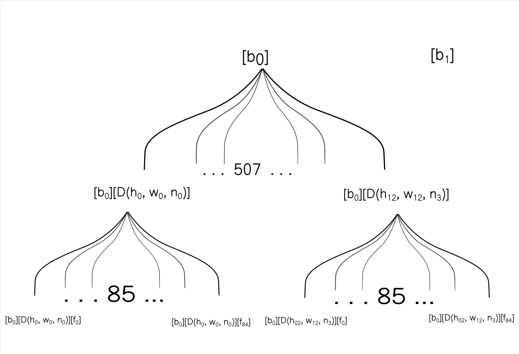
In our target array, the first dimension is the batch. The second dimension is the boxes themselves. Each cell predicts 3 boxes in our case, so our target array will have H x W x 3 or 13 x 13 x 3 = 507 such boxes. In our source array, 3 boxes at, say, an arbitrary location [h,w] is given by [h, w, 0:85], [h, w, 85:170]and [h, w, 170:255] respectively. The same information is described by three rows in our target array.
In the memory, the data of the source array is stored something like this.
Now we would like to visualize how data is stored in the target array. But before that, we would like to introduce some terminology to map information between the source and target arrays.
In the target array, each box represents a row. Row with a index D (h, w, n) represents the box n predicted by grid cell at [h,w] in the source array. The columns in target array are denoted as [f1, f2......fn] representing the features of a box.
Our source array has 4 dimensions, whereas our target array has 3 dimensions. The two dimensions used to represent spatial details of the boxes ( h and w) in the source array are basically rolled into one in the target array.
Therefore, we first begin by flattening out the spatial dimensions in our source array into one.
output = output.reshape(b, c, h * w)
Once this is done, can we simply reshape it to the array to [b, num_boxes, box_width_length] and be done with it? The answer is no. Why? Because we know reshaping would not change how the array is stored in the memory.
In our array (that we just reshaped), we store the information in the following way.
[b0][c0][h0,w0] [b0][c0][h0,w1] [b0][c0][h0,w2] [b0][c0][h0,w3] However, in our target array, two adjacent cells describe two channels for a single cell.
[b0][D(h0, w0, B0)][f1] [b0][D(h0, w0, b0)][f2] [b0][D(h0, w0, b0)][f3] For each batch, and for each spatial location in that batch, store the information across the channels and then move to the other spatial location, and then move to the other batch element.
Note f1....fn is basically the information described along the channel the channel c in the source array. (Refer to the transformation diagram above).
This means that in the internal memory, our source array is stored in a different way in our target array. Reshaping alone can't do the job. Thus, we must modify how arrays are stored.
The fundamental difference between the array we have and the one we want to arrive at is the order of dimensions encoding channel and spatial information. If we take the array we have, and swap the dimensions for the channel and the spatial features dimensions, we would get an array that is stored in the memory like this.
[b0][h0,w0][c0] [b0][h0,w0][c1] [b0][h0,w0][c2] [b0][h0,w0][c3] This is precisely how the information is stored in the target array. This re-order of dimensions can be accomplished by a transpose operation.
output = output.transpose(0, 2, 1)
However, our job is not done yet. We still have the entire channel information in the third dimension of the new array. As stated above, the channel information contains information of three boxes end to end.
The array we have now is of shape [b][h*w][c]. arr[b][h,w] describes three boxes arr[b][h,w][c:c//3], arr[b][h,w][c//3: 2*c//3] and arr[b][h,w][2*c//3:c]. What we want to do is to create an array of shape [b][h*w*3][c/3] such that 3 boxes per channel are accommodated as 3 entries in the second dimension.
Note that the way our current array is stored in memory is same as the way our target array would be.
# Current Array
[b0][h0,w0][c0]   [b0][h0,w0][c1]   [b0][h0,w0][c2]  [b0][h0,w0][c3]

# Destination Array
[b0][D(h0, w0, b0)][f1]  [b0][D(h0, w0, b0)][f2]  [b0][D(h0, w0, b0)][f3]
Therefore, we can easily turn our current array into the destination array using a reshape operation.
output = output.reshape(b, c * h * w // box_info_length, box_info_length)
This finally gives us our desired output without the loop!
Timing the new code
So now that we have a new way to accomplish our task. Let us compare the time taken by the two versions of the code. Let's time the loop version first.
%%timeit -n 1000
counter = 0

b, c, h, w = (conv_map.shape)
box_info_length = 85


counter = 0
output = np.zeros((b, c * h * w // box_info_length, box_info_length))

for x_b in range(b):
    for x_h in range(h):
        for x_w in range(w):
            for x_c in range(0, c, box_info_length):
                output[x_b, counter] = conv_map[x_b, x_c: x_c + box_info_length, x_h, x_w]
                counter += 1

Let us now time the optimized code.
%%timeit -n 1000

output = conv_map[:]

b, c, h, w = (conv_map.shape)
box_info_length = 85

output = output.reshape(b, c, h * w)
output = output.transpose(0, 2, 1)
output = output.reshape(b, c * h * w // box_info_length, box_info_length)
We see that thee optimized code runs in about 18.2 nanoseconds, which is about 20 times faster than the loop version!
Effect on FPS of the Object Detector
While the optimized code runs about 20x faster than the loop version, the actual boost in FPS is about 8x when I use a confidence threshold of 0.75 on my RTX 2060 GPU. The reason why we get a lesser speed-up is because of a few reasons which are mentioned as follows.
First, if the number of objects detected are too many, then the bottleneck of the code becomes drawing the rectangular boxes on the images, and not the output pipeline. Therefore the gains from the output pipeline don't exactly correspond to gains in FPS.
Second, each frame has a different number of boxes. Even the moving average of the frame rate varies throughout the video. Of course even the confidence threshold will affect the frame rate, as a lesser confidence threshold means more boxes detected.
Third, the speed-up you get may vary depending upon what sort of GPU you are using as well.
That's why I have demonstrated the time difference between the snippets of the code and not the detector itself. The speed-up in FPS on the detector will vary on a case-by-case basis depending on the parameters I have talked about above. However, every time I have used this trick, my speed-ups have always been considerable. Even a 5x speed-up in FPS can mean that object detection can be performed real time.
Setting up an object detector can be quite an elaborate exercise, and is beyond the scope of this post, for not all the readers may be into deep learning-based computer vision. For those who are interested, you can check out my YOLO series. That particular implementation uses reshape and transpose to speedup the output pipeline.
Conclusion
That's it for this part folks. In this part, we saw how methods like reshape and transpose can help us speed up information re-arrangement tasks. While transpose does require making a copy, the loop is still moved to the C routines and therefore is faster than transpose implemented using pythonic loops.
While we optimized the output of an object detector, similar ideas can be applied to allied applications like semantic segmentation, pose detection, etc., where a convolutional feature map is our ultimate output. For now, I'm going to put this series to rest. It's my hope that these posts would have helped you to appreciate NumPy better and write more optimized code. Till then, signing off!