So far we've built two major components of our neural architecture search (NAS) pipeline. In the second part of this series we created a model generator which takes encoded sequences and creates MLP models out of them, compiles them, transfers weights from previously trained architectures, and trains the new ones. In the third part of this series we looked at building the controller for our neural architecture search tool, which sampled architecture sequences using an LSTM controller. We also looked at how we can incorporate an accuracy predictor in the controller.
In this final part of the series we will look at how we make those two components work together. We'll cover custom loss functions and how to use the REINFORCE gradient to train our controller. We'll also implement our search logic, and look at some evaluation tools.
Bring this project to life
This tutorial will cover:
- The pipeline
- Training the models
- Logging model metrics
- Data preparation for controller
- REINFORCE gradient
- Training the controller
- Evaluating model metrics
- Understanding the results
The pipeline
As we discussed in the previous parts of the series as well, we see that the overall pipeline involves the following steps -
- Use the controller to generate an encoded sequence that represents a valid MLP architecture.
- Convert the encoded sequence into an actual MLP model.
- Train said MLP model and make a note of its validation accuracy.
- Utilize this validation accuracy and the encoded model architecture to train the controller itself.
- Repeat.
We have already seen how the controller can do #1 and how the model generator can do #2 and #3. We have also written functions for training the controller. But an important part is missing. In our controller, we write functions for training in a manner that takes the loss function, among other things as input.
Before we get into all of that, lets start building our main MLPNAS class. This class inherits the Controller class we wrote in the previous part and also initializes the MLPGenerator class as an object. Both the classes will interact with each other to perform the architecture search.
After importing the constants file, we will initialize it with the following constants -
- number of target classes in the data set.
- how many architectures must be sampled in each controller epoch (imagine this to be a batch size for the controller)
- how many total controller epochs
- how many epochs to train controller on each controller epoch
- how many epochs to train each generated architecture
- the alpha value needed to calculate discounted reward (more about this later)
class MLPNAS(Controller):

    def __init__(self, x, y):

        self.x = x
        self.y = y
        self.target_classes = TARGET_CLASSES
        self.controller_sampling_epochs = CONTROLLER_SAMPLING_EPOCHS
        self.samples_per_controller_epoch = SAMPLES_PER_CONTROLLER_EPOCH
        self.controller_train_epochs = CONTROLLER_TRAINING_EPOCHS
        self.architecture_train_epochs = ARCHITECTURE_TRAINING_EPOCHS
        self.controller_loss_alpha = CONTROLLER_LOSS_ALPHA

        self.data = []
        self.nas_data_log = 'LOGS/nas_data.pkl'
        clean_log()

        super().__init__()

        self.model_generator = MLPGenerator()

        self.controller_batch_size = len(self.data)
        self.controller_input_shape = (1, MAX_ARCHITECTURE_LENGTH - 1)
        if self.use_predictor:
            self.controller_model = self.hybrid_control_model(self.controller_input_shape, self.controller_batch_size)
        else:
            self.controller_model = self.control_model(self.controller_input_shape, self.controller_batch_size)
Training MLP models
The models that we generate using the controller as a sequence have to be converted into MLP models that can be trained and evaluated. These training and evaluation metrics need to be logged since the validation accuracies will feed into our reward function. Besides the real metrics of these models, we also need to predict the validation accuracy of the given sequence if you're using an accuracy predictor.
Assuming the controller is generating the sequence and considering the MLP Generator code we wrote in the second part of the series and initialized in the MLPNAS class above, we can write the creation and training of architectures as mentioned below. We train our generated architectures for classification tasks and use the categorical cross-entropy function unless the number of classes is 2. If that is the case, we use the binary cross-entropy function. We shuffle the data every time a new architecture is about to get trained, and return the history of the trained model. The functions used by the mlp_generator are all covered in the second part of this series.
# create architectures using encoded sequences we got from the controller
def create_architecture(self, sequence):

    # define loss function according to number of target labels
    if self.target_classes == 2:
	    self.model_generator.loss_func = 'binary_crossentropy'

    # create the model using the model generator
    model = self.model_generator.create_model(sequence, np.shape(self.x[0]))

    # compile said model
    model = self.model_generator.compile_model(model)
    return model

# train the generated architecture
def train_architecture(self, model):

    # shuffle the x and y data
    x, y = unison_shuffled_copies(self.x, self.y)

    # train the model
    history = self.model_generator.train_model(model, x, y, self.architecture_train_epochs)
    return history
Before we look into how to log the metrics so we are able to access it easily and so that it captures all the things required for the model, let's look into how the controller fits into the MLPNAS pipeline overall.
Storing the training metrics
While storing the training metrics we need to consider the number of epochs each model was trained for. If it was trained for more than 1 epoch, we take a moving average of the validation accuracies of all epochs. We could use other strategies like giving higher weights to the first few epochs to get rewards such that they will help to optimize for architectures that will learn faster.
If the accuracy predictor is a part of the pipeline, the predicted accuracies are also appended to each MLP model training entry.
    def append_model_metrics(self, sequence, history, pred_accuracy=None):

        # if the MLP models are trained only for a single epoch
        if len(history.history['val_accuracy']) == 1:

            # if an accuracy predictor is used
            if pred_accuracy:
                self.data.append([sequence,
                                  history.history['val_accuracy'][0],
                                  pred_accuracy])

            # if no accuracy predictor data available
            else:
                self.data.append([sequence,
                                  history.history['val_accuracy'][0]])
            print('validation accuracy: ', history.history['val_accuracy'][0])

        # if the MLP models are trained for more than one epoch
        else:

            # take a moving average of validation accuracy across epochs
            val_acc = np.ma.average(history.history['val_accuracy'],
                                    weights=np.arange(1, len(history.history['val_accuracy']) + 1),
                                    axis=-1)

            # add predicted accuracies if available else don't
            if pred_accuracy:
                self.data.append([sequence,
                                  val_acc,
                                  pred_accuracy])
            else:
                self.data.append([sequence,
                                  val_acc])
            print('validation accuracy: ', val_acc)
Preparing data for controller
We train the controller on encoded sequences by padding sequences, splitting them into inputs and labels by separating the last element in each sequence from the rest of the sequence.
We also return validation accuracies for those sequences as they will help us determine the reward for the controller training and also the target for the accuracy predictor. This data is acquired from the self.data list we initialized in the MLPNAS class and populated as detailed in the previous section.
    def prepare_controller_data(self, sequences):

        # pad generated sequences to maximum length
        controller_sequences = pad_sequences(sequences, maxlen=self.max_len, padding='post')

        # split into inputs and labels for LSTM controller
        xc = controller_sequences[:, :-1].reshape(len(controller_sequences), 1, self.max_len - 1)
        yc = to_categorical(controller_sequences[:, -1], self.controller_classes)

        # get validation accuracies for each for reward function
        val_acc_target = [item[1] for item in self.data]
        return xc, yc, val_acc_target
Using the REINFORCE Gradient
As we have seen in the first part of the series, there are several ways a controller can be optimized - genetic algorithms, game theory, etc. In this implementation we will utilize something called the REINFORCE gradient.
REINFORCE gradient is a policy optimization method that leverages Monte Carlo sampling and expected rewards optimization to move towards better results.
In our NAS framework we can assume the state to be the state of the LSTM controller, the actions to be the next element in the sequence as predicted by said controller, and the policy being the probability distribution that determines the action, given the state. If you remember the function we wrote for sampling the next element of a sequence given the previous ones, you will see that the probability array (softmax distribution) we get after feeding our LSTM with previous sequences as input is the policy. We use probabilistic sampling to get our action. The probabilistic sampling encourages exploration.
REINFORCE gradient is a way to optimize policy gradients.
This article gives a comprehensive guide to deriving the REINFORCE gradient. The overview of the method is shown below -
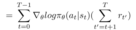
The Probability term which corresponds to the policy of our network can be split into its corresponding terms using conditional probability, apply a log function and differentiated with respect to the parameters.
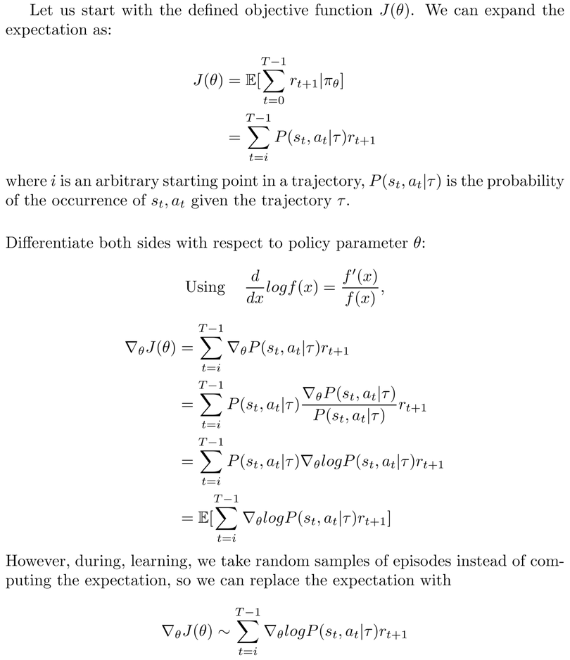
This gives us the following result:
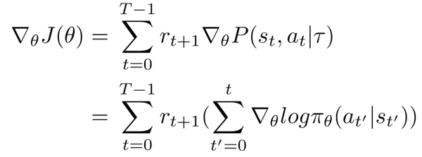
Here pi represents the policy at parameters theta.
We expand the result and finally arrive at the following result -
The left side of the expression is the log likelihood of the policy (represented by pi) given the action a in state s corresponding to time t, or the controller's softmax distribution.
The right side of the expression (the summation in parentheses) is the term that is looking at the rewards our agent gets. We want to incorporate a discount factor in our expression to award greater weight to immediate rewards compared to the future ones. The term on the right, the reward sum term starting from t till the episode ends is for this purpose multiplied by a gamma term which is raised to an exponent equal to t' - t - 1.
The final expression hence becomes
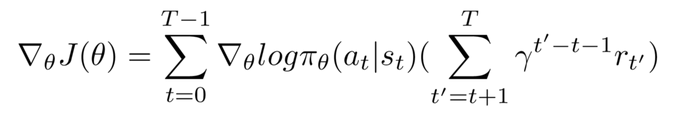
where the summation on the right end of the right hand side of the equation is the discounted reward.
Implementing REINFORCE Gradient
To implement the REINFORCE gradient we write a custom loss function that implements the above mentioned product of log-probabilities and the discounted reward.
We define a function to calculate the discounted reward, which iteratively adds the gamma value raised to the counter and multiplied with the reward at that step. The number of iterative additions is dependent on the value of t for that particular action. After acquiring the discounted rewards, we normalize it according to its z values (calculated by subtracting the mean and dividing by the standard deviation) and use this array as the discounted rewards in our custom loss function.
The discounted rewards themselves depend on the rewards, which we define as the validation accuracy of a particular network from which a baseline is subtracted. Having a baseline (in our case, 0.5) makes sure that networks with less than 50% accuracy are punished and the ones above 50% are rewarded. Of course you can change this value in favor of a higher accuracy in your own implementation.
    def get_discounted_reward(self, rewards):

        # initialise discounted reward array
        discounted_r = np.zeros_like(rewards, dtype=np.float32)

        # every element in the discounted reward array
        for t in range(len(rewards)):
            running_add = 0.
            exp = 0.

            # will need us to iterate over all rewards from t to T
            for r in rewards[t:]:
                running_add += self.controller_loss_alpha**exp * r
                exp += 1

            # add values to the discounted reward array
            discounted_r[t] = running_add

        # normalize discounted reward array
        discounted_r = (discounted_r - discounted_r.mean()) / discounted_r.std()
        return discounted_r

	# loss function based on discounted reward for policy gradients
    def custom_loss(self, target, output):

        # define baseline for rewards and subtract it from all validation accuracies to get reward.
        baseline = 0.5
        reward = np.array([item[1] - baseline for item in self.data[-self.samples_per_controller_epoch:]]).reshape(
            self.samples_per_controller_epoch, 1)

        # get discounted reward
        discounted_reward = self.get_discounted_reward(reward)

        # multiply discounted reward by log likelihood of actions to get loss function
        loss = - K.log(output) * discounted_reward[:, None]
        return loss
While writing a custom loss function in Keras, we have to make sure that the inputs are always the target and the output even though we will not be using any target values for the purpose of training our controller. We get the negative log of the outputs (softmax distribution of possible actions) and multiply it with the discounted rewards. This loss function is then optimized in our training processes by whichever optimizer we choose.
Training the controller
Once we have the loss function, the only thing we need to be concerned about when training the controller is if the controller is using an accuracy predictor. If it is, we use the hybrid control model we defined in the third part of the series. If not, we use the simple control model.
The hybrid controller will take the predicted accuracies as inputs as well. We do not write a separate loss function for the accuracy predictor. Instead a mean squared error loss is used for the accuracy predictor.
    def train_controller(self, model, x, y, pred_accuracy=None):
        if self.use_predictor:
            self.train_hybrid_model(model,
                                    x,
                                    y,
                                    pred_accuracy,
                                    self.custom_loss,
                                    len(self.data),
                                    self.controller_train_epochs)
        else:
            self.train_control_model(model,
                                     x,
                                     y,
                                     self.custom_loss,
                                     len(self.data),
                                     self.controller_train_epochs)
The Main NAS loop
We have written all the functionalities that are required to finally run the entire NAS pipeline.
The main function looks something like this:
    def search(self):

        # for every controller epoch
        for controller_epoch in range(self.controller_sampling_epochs):

            # generate sequences
            sequences = self.sample_architecture_sequences(self.controller_model, self.samples_per_controller_epoch)

            # if using a predictor, predict their accuracies
            if self.use_predictor:
                pred_accuracies = self.get_predicted_accuracies_hybrid_model(self.controller_model, sequences)

            # for each sequence generated in a controller epoch
            for i, sequence in enumerate(sequences):

                # create an MLP model
                model = self.create_architecture(sequence)

                # train said MLP model
                history = self.train_architecture(model)

                # log the model metrics
                if self.use_predictor:
                    self.append_model_metrics(sequence, history, pred_accuracies[i])
                else:
                    self.append_model_metrics(sequence, history)

            # prepare data for the controller
            xc, yc, val_acc_target = self.prepare_controller_data(sequences)

            # train the controller
            self.train_controller(self.controller_model,
                                  xc,
                                  yc,
                                  val_acc_target[-self.samples_per_controller_epoch:])

        # save all the NAS logs in a pickle file
        with open(self.nas_data_log, 'wb') as f:
            pickle.dump(self.data, f)

        return self.data
The Constants
There are a lot of parameters that one might have to vary while experimenting with the performance of our NAS method. To make the constants more accessible, we create a separate file which will hold all the necessary parameters. You may have noticed that all the scripts we have written until now utilize certain initialization values. These values will be imported from the constant file we define below.
########################################################
#                   NAS PARAMETERS                     #
########################################################
CONTROLLER_SAMPLING_EPOCHS = 10
SAMPLES_PER_CONTROLLER_EPOCH = 10
CONTROLLER_TRAINING_EPOCHS = 10
ARCHITECTURE_TRAINING_EPOCHS = 10
CONTROLLER_LOSS_ALPHA = 0.9

########################################################
#               CONTROLLER PARAMETERS                  #
########################################################
CONTROLLER_LSTM_DIM = 100
CONTROLLER_OPTIMIZER = 'Adam'
CONTROLLER_LEARNING_RATE = 0.01
CONTROLLER_DECAY = 0.1
CONTROLLER_MOMENTUM = 0.0
CONTROLLER_USE_PREDICTOR = True

########################################################
#                   MLP PARAMETERS                     #
########################################################
MAX_ARCHITECTURE_LENGTH = 3
MLP_OPTIMIZER = 'Adam'
MLP_LEARNING_RATE = 0.01
MLP_DECAY = 0.0
MLP_MOMENTUM = 0.0
MLP_DROPOUT = 0.2
MLP_LOSS_FUNCTION = 'categorical_crossentropy'
MLP_ONE_SHOT = True

########################################################
#                   DATA PARAMETERS                    #
########################################################
TARGET_CLASSES = 3

########################################################
#                  OUTPUT PARAMETERS                   #
########################################################
TOP_N = 5
The only thing that you have to necessarily change when switching from one dataset to another is the number of target classes present in the dataset.
Running MLPNAS
That's it. Now all we have to do is run the algorithm for a dataset of our choice! This is what the final file - run.py - looks like.
import pandas as pd

from utils import *
from mlpnas import MLPNAS
from CONSTANTS import TOP_N

# read the data
data = pd.read_csv('DATASETS/wine-quality.csv')

# split it into X and y values
x = data.drop('quality_label', axis=1, inplace=False).values
y = pd.get_dummies(data['quality_label']).values

# let the search begin
nas_object = MLPNAS(x, y)
data = nas_object.search()

# get top n architectures (the n is defined in constants)
get_top_n_architectures(TOP_N)
As you can see, we have a final function to get top n architectures we haven't yet detailed.
Evaluation and Visualization
Some basic visualisations and evaluations can be done when looking through all the data we get from our architecture search. For the purpose of this article, we will try to understand:
- What are the best architectures, and what are the accuracies they promise?
- How did the accuracies progress over the controller iterations?
- What is the distribution of accuracies in the architectures we tested in the search?
We can see the most recent logs by using mtime in Python. We can also isolate the latest event ID and accordingly retrieve the NAS data for our latest run.
def get_latest_event_id():
    all_subdirs = ['LOGS/' + d for d in os.listdir('LOGS') if os.path.isdir('LOGS/' + d)]
    latest_subdir = max(all_subdirs, key=os.path.getmtime)
    return int(latest_subdir.replace('LOGS/event', ''))
Once you have the latest event ID, you can load and sort the data according to the validation accuracies to find which ones did better than the others.
########################################################
#                 RESULTS PROCESSING                   #
########################################################


def load_nas_data():
    event = get_latest_event_id()
    data_file = 'LOGS/event{}/nas_data.pkl'.format(event)
    with open(data_file, 'rb') as f:
        data = pickle.load(f)
    return data


def sort_search_data(nas_data):
    val_accs = [item[1] for item in nas_data]
    sorted_idx = np.argsort(val_accs)[::-1]
    nas_data = [nas_data[x] for x in sorted_idx]
    return nas_data
You can utilize this sorted data to find out what the top n architectures are. You can also use the stored data to find what the encoded architecture sequences look like when decoded, and what their validation accuracies were.
def get_top_n_architectures(n):
    data = load_nas_data()
    data = sort_search_data(data)
    search_space = MLPSearchSpace(TARGET_CLASSES)
    print('Top {} Architectures:'.format(n))
    for seq_data in data[:n]:
        print('Architecture', search_space.decode_sequence(seq_data[0]))
        print('Validation Accuracy:', seq_data[1])
Here's an example of the output of a run which utilized the one-shot architecture method, but not the accuracy predictor.
Architecture [(128, 'relu'), (3, 'softmax')]
Validation Accuracy: 0.7023747715083035
Architecture [(512, 'relu'), (3, 'softmax')]
Validation Accuracy: 0.6857143044471741
Architecture [(512, 'sigmoid'), (64, 'sigmoid'), (3, 'softmax')]
Validation Accuracy: 0.6775510311126709
Architecture [(32, 'elu'), (3, 'softmax')]
Validation Accuracy: 0.6745825615796176
Architecture [(8, 'elu'), (16, 'tanh'), (3, 'softmax')]
Validation Accuracy: 0.6664564111016014
The results can vary with random number generator seeds and it is advisable to set the seed before running these algorithms to get reproducible results. These results are obtained after training 100 architectures and training the controller after every 10 architectures. Running the algorithm longer and testing more architectures would yield better results.
Other things can be uncovered about the nature of our search by looking at the raw, non-sorted data. In the first function below, get_nas_accuracy_plot(), we plot the accuracies as they changed over several iterations.
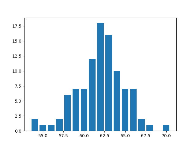
In the second one, get_accuracy_distribution(), we bin our accuracies by their closest integer values and get a bar plot of the number of architectures that fall into different integer bins, ranging from 0 to 100.
def get_nas_accuracy_plot():
    data = load_nas_data()
    accuracies = [x[1] for x in data]
    plt.plot(np.arange(len(data)), accuracies)
    plt.show()


def get_accuracy_distribution():
    event = get_latest_event_id()
    data = load_nas_data()
    accuracies = [x[1]*100. for x in data]
    accuracies = [int(x) for x in accuracies]
    sorted_accs = np.sort(accuracies)
    count_dict = {k: len(list(v)) for k, v in groupby(sorted_accs)}
    plt.bar(list(count_dict.keys()), list(count_dict.values()))
    plt.show()
The same run provided me with the following accuracy distributions.
The above mentioned functions are only meant to get you started on evaluating NAS methods. You could define more evaluation methods as well, like trying to understand model prediction by finding out which layers were predicted to be the first layer or the second layer, which hidden layer impacted the accuracies the most, etc.
Conclusion
This brings us to the end of our 4-part series. In Part 1 we saw a thorough overview of where the Neural Architecture Search research is at currently. We saw how NAS works in broader terms works, what are the different approaches that people have classically used to solve the problem, what are the lesser-known approaches for the same problems, how they perform, etc. We also looked at several papers tackling the important problem of computational efficiency for NAS algorithms.
In Part 2 we tackle the simpler problem of designing MLPs automatically as an implementation exercise. We build our search space and a generator that will take an encoded sequence as designed in the search space and convert it into Keras architectures that can be trained and evaluated. We also explore one-shot learning.
Part 3 deals with controllers, the mechanism that generates these encoded sequences to start with. Besides building an LSTM controller, we also look at accuracy predictions and how they can be tied together in a hybrid controller model.
Finally, we tied all of these pieces together in this article by implementing REINFORCE gradient as the controller optimization method. We also looked at some NAS evaluation techniques. We look at implementing custom loss functions, understanding discounted rewards, and stitching it all together to run the search in just a few final lines of code. We also look into some basic ways of visualizing and analyzing the results we get from NAS for MLPs.
The complete code implementation can be found here.
I hope you enjoyed the series.