The aim of this three-part series has been to shed light on the landscape and development of deep learning models that have defined the field and improved our ability to solve challenging problems. In Part 1 we covered models developed from 2012-2014, namely AlexNet, VGG16, and GoogleNet. In Part 2 we saw more recent models from 2015-2016: ResNet, InceptionV3, and SqueezeNet. Now that we've covered the popular architectures and models of the past, we'll move on to the state of the art.
The architectures that we'll discuss here include:
- DenseNet
- ResNeXt
- MnasNet
- ShuffleNet v2
Let's get started.
Bring this project to life
DenseNet (2016)
The name “DenseNet” refers to Densely Connected Convolutional Networks. It was proposed by Gao Huang, Zhuang Liu, and their team in 2017 at the CVPR Conference. It received the best paper award, and has accrued over 2000 citations.
Traditional convolutional networks with n layers have n connections; one between each layer and its subsequent layer. In DenseNet each layer connects to every other layer in a feed-forward fashion, meaning that DenseNet has n(n+1)/2 connections in total. For each layer the feature maps of all preceding layers are used as inputs, and its own feature-maps are used as inputs to all subsequent layers.
Dense Blocks
DenseNet boasts one big advantage over conventional deep CNNs: the information passed through many layers will not be washed-out or vanish by the time it reaches the end of the network. This is achieved by a simple connectivity pattern. To understand this, one must know how layers in a normal CNN are connected.
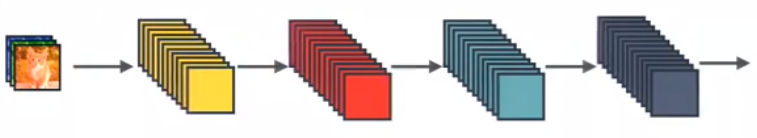
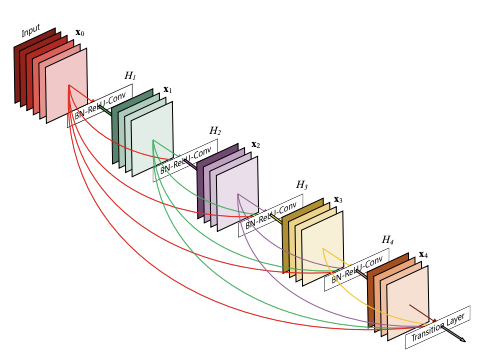
Here’s a simple CNN where the layers are sequentially connected. In the Dense Block, however, each layer obtains additional inputs from all preceding layers, and passes its own feature maps to all subsequent layers. Below is an image depicting the dense block.

As the layers in the network receive feature maps from all the preceding layers, the network will be thinner and more compact. Below is a 5-layer dense block with the number of channels set to 4.
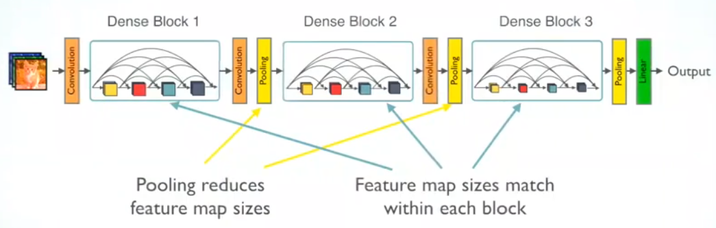
The DenseNet Architecture
DenseNet has been applied to various different datasets. Based on the dimensionality of the input, different types of dense blocks are used. Below is a brief description of these layers.
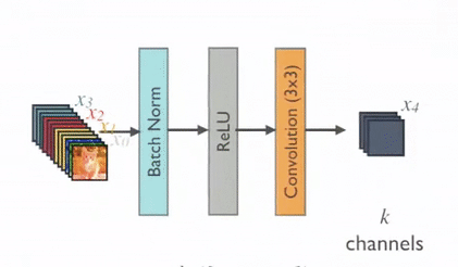
- Basic DenseNet Composition Layer: In this type of dense block each layer is followed by a pre-activated batch normalization layer, ReLU activation function, and a 3×3 convolution. Below is a snapshot.
- BottleNeck DenseNet (DenseNet-B): As every layer produces k output feature maps, computation can be harder at every level. Hence the authors presented a bottleneck structure where 1×1 convolutions are used before a 3×3 convolution layer, shown below.
- DenseNet Compression: To improve the model compactness, the authors tried reducing the feature maps at the transition layers. So if a dense block consists of m feature maps and the transition layer generates i output feature maps, where 0 < i <= 1, this i also denotes the compression factor. If the value of i is equal to one (i=1), the number of feature maps across transition layers remains unchanged. If i < 1, then the architecture is referred to as DenseNet-C and the value of i would be changed to 0.5. When both the bottleneck and transition layers with i < 1 are used, we refer to our model as DenseNet-BC.
- Multiple Dense Blocks with Transition Layers: The dense blocks in the architecture are followed by a 1×1 Convolution layer and 2×2 average pooling layer. As the feature map sizes are the same, it’s easy to concatenate the transition layers. Lastly, at the end of the dense block, a global average pooling is performed which is attached to a softmax classifier.
DenseNet Training and Results
The DenseNet architecture defined in the original research paper is applied to three datasets: CIFAR, SVHN, and ImageNet. All the architectures used a stochastic gradient descent optimizer for training. The training batch size for CIFAR and SVHN was 64, for 300 and 40 epochs, respectively. The initial learning rate was set to 0.1 and was further reduced. Below are the metrics for DenseNet trained on ImageNet:
- Batch size: 256
- Epochs: 90
- Learning rate: 0.1, decreased by a factor of 10 at epochs 30 and 60
- Weight decay and momentum: 0.00004 and 0.9
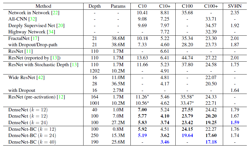
Below are the detailed results showing how different configurations of DenseNet compare to other networks on the CIFAR and SVHN datasets. The data in blue indicates the best results.
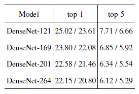
Below are the Top-1 and Top-5 errors for different sizes of DenseNet on ImageNet.
Below are a few relevant links if you want to look into the original paper, its implementation, or how to implement DenseNet yourself:
- Most of the images in this review are taken from the original research paper (DenseNet) and the article Review: DenseNet — Dense Convolutional Network (Image Classification) by Sik-Ho Tsang
- Code corresponding to the original paper
- TensorFlow Implementation of DenseNet
- PyTorch Implementation of DenseNet
ResNeXt (2017)
ResNeXt is a homogeneous neural network which reduces the number of hyperparameters required by conventional ResNet. This is achieved by their use of "cardinality", an additional dimension on top of the width and depth of ResNet. Cardinality defines the size of the set of transformations.
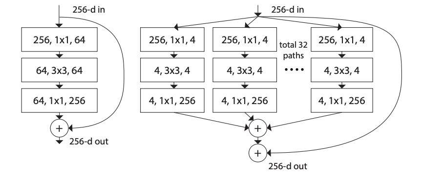
In this image the leftmost diagram is a conventional ResNet block; the rightmost is the ResNeXt block, which has a cardinality of 32. The same transformations are applied 32 times, and the result is aggregated at the end. This technique was suggested in the 2017 paper Aggregated Residual Transformations for Deep Neural Networks, co-authored by Saining Xie, Ross Girshick, Piotr Dollar, Zhuowen Tu, and Kaiming He, who all worked under Facebook AI Research.
VGG-nets, ResNets, and Inception Networks have gained a lot of momentum in the field of feature engineering. Despite their great performances, they still face a handful of limitations. These models are well-suited for several datasets, but due to the many hyperparameters and computations involved, adapting them to new datasets is no minor task. To overcome such issues, the advantages of both VGG/ResNet (ResNet evolved from VGG) and Inception Networks have been considered. In a nutshell, the repetition strategy of ResNet is combined with the split-transform-merge strategy of Inception Network. In other words, a network block splits the input, transforms it into a required format, and merges it to get the output where each block follows the same topology.
ResNeXt Architecture
The basic architecture of ResNeXt is defined by two rules. First, if the blocks produce same-dimensional spatial maps, they share the same set of hyperparameters, and if at all the spatial map is downsampled by a factor of 2, the width of the block is multiplied by a factor of 2.
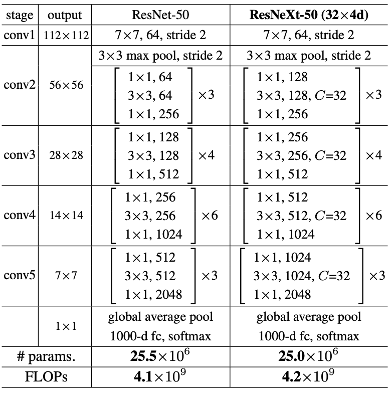
As seen in the table, ResNeXt-50 has 32 as its cardinality repeated 4 times (depth). The dimensions in [] denote the residual block structures, whereas the numbers written adjacent to them refer to the number of stacked blocks. 32 precisely denotes that there are 32 groups in the grouped convolution.
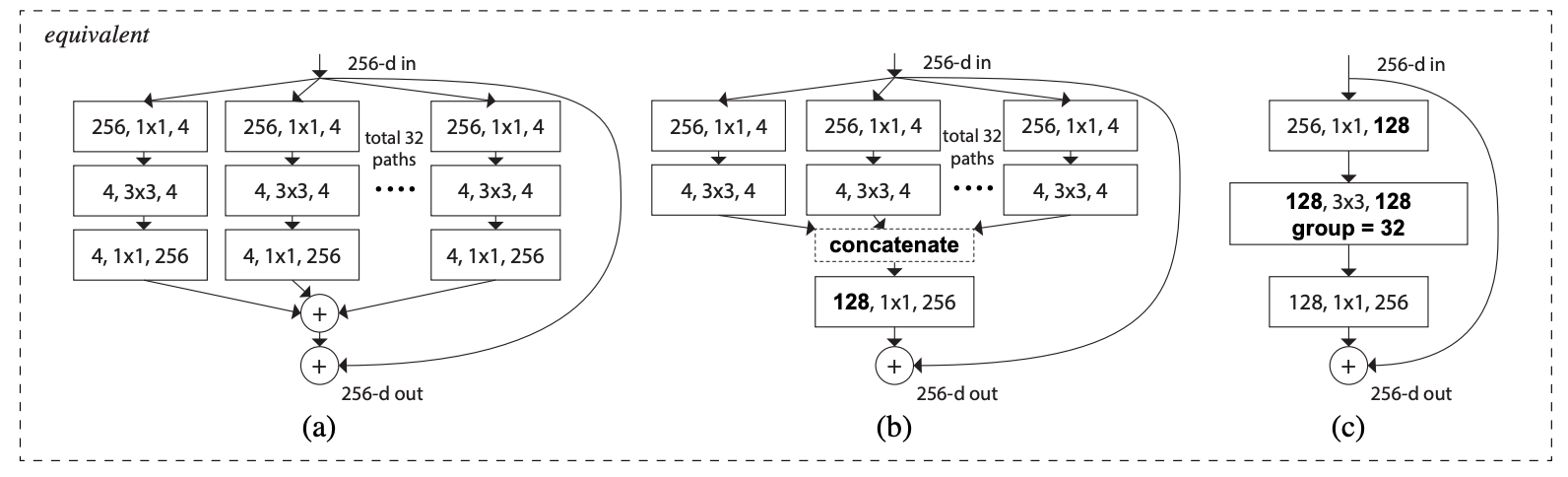
The above network structures explain what a grouped convolution is, and how it trumps the other two network structures.
- (a) denotes a usual ResNeXt block that has already been seen previously. It has a cardinality of 32, and follows the split-transform-merge strategy.
- (b) does seem to be a leaf taken out of Inception-ResNet. However, Inception or Inception-ResNet doesn’t have network blocks following the same topology.
- (c) is related to the grouped convolution which has been proposed in AlexNet architecture. 32*4 as has been seen in (a) and (b) has been replaced with 128 in-short, meaning splitting is done by a grouped convolutional layer. Similarly, the transformation is done by the other grouped convolutional layer that does 32 groups of convolutions. Later, concatenation happens.
Among the above three, (c) proved to be the best as it is simple to implement.
ResNeXt Training and Results
ImageNet has been used to show the enhancement in accuracy when cardinality is considered rather than width/depth.
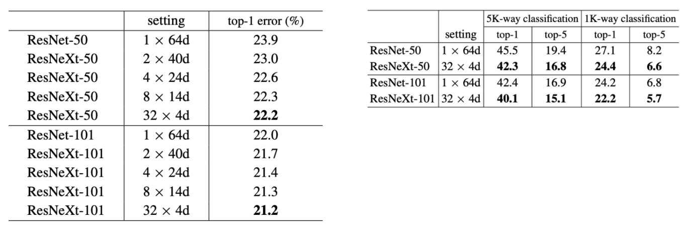
Both ResNeXt-50 and ResNeXt-101 are less error-prone when the cardinality is high. Also, in comparison to ResNet, ResNeXt performed well.
Below are a few important links,
- Link to Original Research Paper
- PyTorch Implementation of ResNext
- Tensorflow Implementation of ResNext
ShuffleNet v2 (2018)
ShuffleNet v2 considers direct metrics, such as speed or memory access cost, to measure the network’s computational complexity (besides FLOPs, which acts as an indirect metric). Moreover, the direct metrics are also evaluated on the target platform. ShuffleNet v2 was thus introduced in the paper, ShuffleNet V2: Practical Guidelines for Efficient CNN Architecture Design, published in 2018. It was co-authored by Ningning Ma, Xiangyu Zhang, Hai-Tao Zheng, and Jian Sun.
FLOPs is the usual metric to measure the performance of a network, in terms of its computations. However, a few studies have substantiated the fact that FLOPs do not wholly dig the underlying truths; networks having similar FLOPs differ in their speeds, this can be because of the memory access cost, degree of parallelism, target platform, etc. All these do not fall under FLOPs, and thus, are being ignored. ShuffleNet v2 overcomes such hassles by proposing four guidelines to model a network.
ShuffleNet v2 Architecture
Prior to understanding the network architecture, the guidelines upon which the network has been built shall give a glimpse into how various other direct metrics have been considered:
- Equal channel width minimizes the memory access cost: When the number of input channels and output channels are in the same proportion (1:1), memory access cost becomes low.
- Excessive group convolution increases memory access cost: The group number shouldn’t be too high, otherwise the memory access cost tends to increase.
- Network fragmentation reduces degree of parallelism: Fragmentation reduces the network’s efficiency in executing parallel computations.
- Element-wise operations are non-negligible: Element-wise operations have small FLOPs, but can increase the memory access time.
All these are integrated in the ShuffleNet v2 architecture to improve the network efficiency.
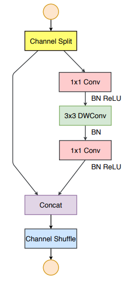
The channel split operator divides the channels into two groups, where one remains as an identity (3rd guideline). The other branch has an equal number of input and output channels along the three convolutions (1st guideline). The 1x1 convolutions aren’t group-wise (2nd guideline). Element-wise operations like ReLU, Concat, depth-wise convolutions are confined to a single branch (4the guideline).
The overall ShuffleNet v2 architecture is tabulated as follows:

The results are with respect to different variations of the output channels.
ShuffleNet v2 Training and Results
Imagenet has been used as the dataset to derive results with various datasets.
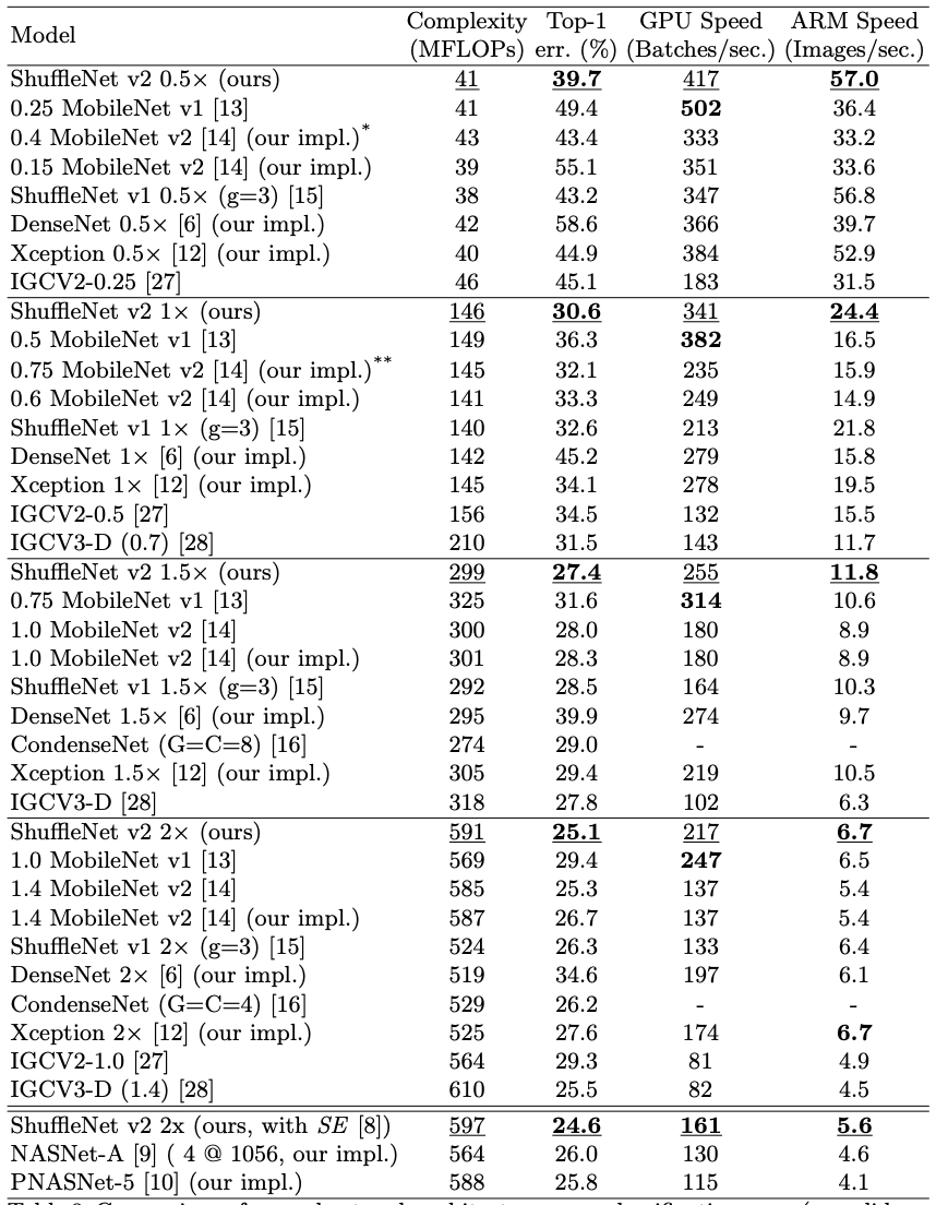
Complexity, error rate, GPU speed, and ARM speed have been used to derive the robust and efficient model among the contemplated models. Although ShuffleNet v2 lacks GPU speed, it records the lowest top-1 error rate, which outweighs the other limitations.
Below are a few additional links which might interest you for implementing ShuffleNet yourself, or diving into the original paper.
- Link to Original Research Paper
- Tensorflow Implementation of ShuffleNet v2
- PyTorch Implementation of ShuffleNet V2
MnasNet (2019)
MnasNet is an automated mobile neural architecture search network that is used to build mobile models using reinforcement learning. It incorporates the basic essence of CNN and thereby strikes the right balance between enhancing accuracy and reducing latency, to depict high performance when the model is deployed onto a mobile. This idea was put forth in the paper, MnasNet: Platform-Aware Neural Architecture Search for Mobile, that came out in 2019. It was co-authored by Mingxing Tan, Bo Chen, Ruoming Pang, Vijay Vasudevan, Mark Sandler, Andrew Howard, and Andrew Howard–all belonging to the Google Brain team.
The conventional mobile CNN models that have been developed so far, do not yield the right outcome when latency and accuracy are taken into account; they somehow lack in either of those. The latency is often estimated using FLOPS, which doesn’t output the right results. However, in MnasNet, the model is directly deployed onto a mobile, and the results are estimated; there are no proxies involved. Mobiles are usually resource-constrained, therefore, factors such as performance, cost, and latency are significant metrics to be considered.
MnasNet Architecture
The architecture, in general, consists of two phases - search space and reinforcement learning approach.
- Factorized hierarchical search space: The search space supports diverse layer structures to be included throughout the network. The CNN model is factorized into various blocks wherein each block has a unique layer architecture. The connections are chosen such that both the input and output are compatible with each other, and henceforth yield good results to maintain a higher accuracy rate. Below is how a search space looks like:
As can be noticed, there are several blocks that make-up for the search space. All the layers are segregated based on their dimensions and filter size. Each block has a specific set of layers where the operations are chosen (as mentioned in blue color). The first layer in every block has a stride 2 if input or output dimensions are different, and the stride is 1 for the remaining layers. The same set of operations is repeated starting from the second layer to the Nth layer where N is the block number.
- Reinforcement search algorithm: As we have two major objectives to achieve - latency and accuracy, we employ a reinforcement learning approach where the rewards are maximized (multi-objective reward). Each CNN model as defined in the search space would be mapped to a sequence of actions that are to be performed by a reinforcement learning agent.
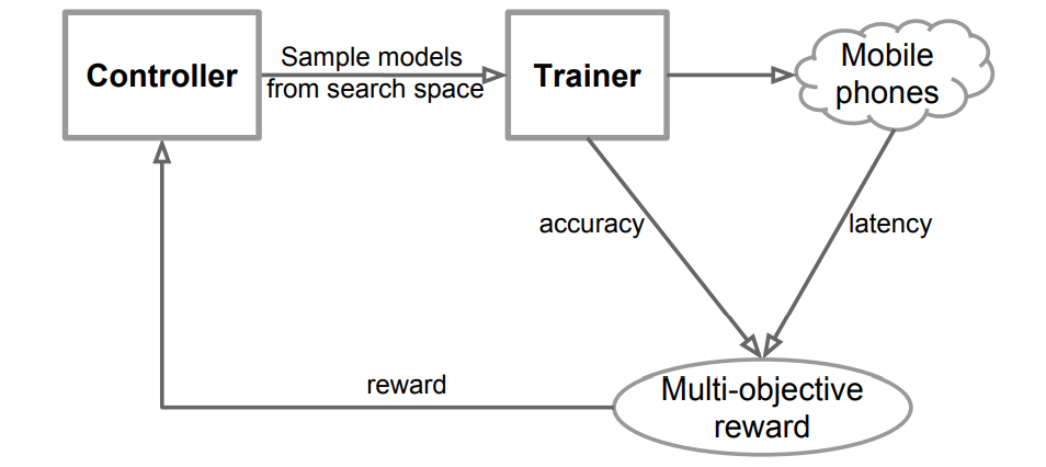
This is what is present in the search algorithm - the controller is a Recurrent Neural Network (RNN), and the trainer trains the model and outputs the accuracy. The model is deployed onto a mobile phone to estimate the latency. Both accuracy and latency are consolidated into a multi-objective reward. This reward is sent to RNN using which the parameters of RNN are updated, to maximize the total reward.
MnasNet Training and Results
Imagenet has been used to depict the accuracy achieved by a MnasNet model, in comparison with the other conventional mobile CNN models. Here’s a table representing the same:
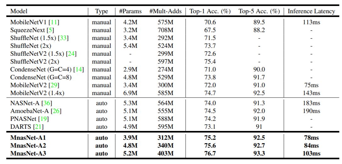
MnasNet definitely has a reduced latency along with improved accuracy.
If you want to check out the original paper or implement MnasNet yourself in PyTorch, check out these links:
That wraps up our three-part series covering popular deep learning architectures that have defined the field. If you haven't already, feel free to check out Part 1 and Part 2, which cover models like ResNet, Inception v3, AlexNet, and others. I hope you found this series useful.