A Review of Popular Deep Learning Architectures: ResNet, InceptionV3, and SqueezeNet

Previously we looked at the field-defining deep learning models from 2012-2014, namely AlexNet, VGG16, and GoogleNet. This period was characterized by large models, long training times, and difficulties carrying over to production.

In this article we’ll dive deep into the models that came after this period, in 2015-2016. Big advancements were made in just these two years, leading to boosts in accuracy and performance. Specifically, we'll look at:

• ResNet
• Wide ResNet
• InceptionV3
• SqueezeNet

Let's get started.

ResNet (2015)

As deep neural networks are both time-consuming to train and prone to overfitting, a team at Microsoft introduced a residual learning framework to improve the training of networks that are substantially deeper than those used previously. This research was published in the paper titled Deep Residual Learning for Image Recognition in 2015. And so, the famous ResNet (short for "Residual Network") was born.

When training deep networks there comes a point where an increase in depth causes accuracy to saturate, then degrade rapidly. This is called the "degradation problem." This highlights that not all neural network architectures are equally easy to optimize.

ResNet uses a technique called "residual mapping" to combat this issue. Instead of hoping that every few stacked layers directly fit a desired underlying mapping, the Residual Network explicitly lets these layers fit a residual mapping. Below is the building block of a Residual network.

The formulation of F(x)+x can be realized by feedforward neural networks with shortcut connections.

Many problems can be addressed using ResNets. They are easy to optimize and achieve higher accuracy when the depth of the network increases, producing results that are better than previous networks. Like its predecessors which we covered in Part 1, ResNet was first trained and tested on ImageNet's over 1.2 million training images belonging to 1000 different classes.

ResNet Architecture

Compared to the conventional neural network architectures, ResNets are relatively easy to understand. Below is the image of a VGG network, a plain 34-layer neural network, and a 34-layer residual neural network. In the plain network, for the same output feature map, the layers have the same number of filters. If the size of output features is halved the number of filters is doubled, making the training process more complex.

Meanwhile in the Residual Neural Network, as we can see, there are far fewer filters and lower complexity during the training with respect to VGG. A shortcut connection is added that turns the network into its counterpart residual version. This shortcut connection performs identity mapping, with extra zero entries padded for increasing dimensions. This option introduces no additional parameter. The projection shortcut is mathematically represented as F(x{W}+x), which is used to match dimensions computed by 1×1 convolutions.

Below is the table showing the layers and parameters in the different ResNet Architectures.

Each ResNet block is either two layers deep (used in small networks like ResNet 18 or 34), or 3 layers deep (ResNet 50, 101, or 152).

ResNet Training and Results

The samples from the ImageNet dataset are re-scaled to 224 × 224 and are normalized by a per-pixel mean subtraction. Stochastic gradient descent is used for optimization with a mini-batch size of 256. The learning rate starts from 0.1 and is divided by 10 when the error increases, and the models are trained up to 60 × 104 iterations. The weight decay and momentum are set to 0.0001 and 0.9 respectively. Dropout layers are not used.

ResNet performs extremely well with deeper architectures. Below is an image showing the error rate of two 18 and 34-layer neural networks. On the left the graph shows plain networks, while the graph on the right shows their ResNet equivalents. The thin red curve in the image represents the training error, and the bold curve represents the validation error.

Below is the table showing the Top-1 error (%, 10-crop testing) on ImageNet validation.

ResNet has played a significant role in defining the field of deep learning as we know it today.

Below are a few important links if you're interested in implementing a ResNet yourself:

1. PyTorch ResNet Implementation
2. Tensorflow ResNet Implementation
3. Link to the Original Research Paper

Wide ResNet (2016)

The Wide Residual Network is a more recent improvement on the original Deep Residual Networks. Rather than relying on increasing the depth of a network to improve its accuracy, it was shown that a network could be made shallower and wider without compromising its performance. This ideology was presented in the paper Wide Residual Networks, which was published in 2016 (and updated in 2017 by Sergey Zagoruyko and Nikos Komodakis.

Deep Residual Networks have shown remarkable accuracies that have aided in performing tasks like image recognition, among many others, with relative ease. Nonetheless, a deep network still faces the challenges of network degradation as well as exploding or vanishing gradients. A deep residual network doesn’t guarantee the usage of all residual blocks either; just a few could be skipped, or only a few make it to the larger contributing blocks (i.e. extract useful information). This problem could be solved by disabling random blocks–this is dropout in a broader sense. Taking a cue from this idea, the authors of Wide ResNet have proved that a wide residual network can perform even better than a deep one.

Wide ResNet Architecture

A Wide ResNet has a group of ResNet blocks stacked together, where each ResNet block follows the BatchNormalization-ReLU-Conv structure. This structure is depicted as follows:

There are five groups that comprise a wide ResNet. The block here refers to the residual block B(3, 3). Conv1 remains intact in any network, whereas conv2, conv3, and conv4 vary according to k, a value that defines the width. The convolutional layers are succeeded by an average-pool layer and a classification layer.

The following variable measures could be tweaked to come up with various representations of the residual blocks:

• Convolution type: B(3, 3) shown above has 3 × 3 convolutional layers in the residual block. Other possibilities, such as integrating 3 × 3 convolutional layers with 1 × 1 convolutions, could be explored as well.
• Convolutions per block: The depth of the block has to be determined by estimating the dependency of this metric on the performance of the model.
• Width of residual blocks: The width and depth have to be checked consistently to keep an eye on both computational complexity and performance.
• Dropout: A dropout layer should be added between convolutions in every residual block. This prevents overfitting.

Wide ResNet Training and Results

Wide ResNet was trained on CIFAR-10. The following metrics resulted in the lowest error rates:

• Convolution type: B(3, 3)
• Convolution layers per residual block: 2. Thus B(3,3) was the preferred dimension (rather than B(3, 3, 3) or B(3, 3, 3, 3), for instance).
• Width of residual blocks: A depth of 28 and a width of 10 seemed to be less error-prone.
• Dropout: When dropout was included the error rate was further reduced. The comparative results are shown in the figure below.

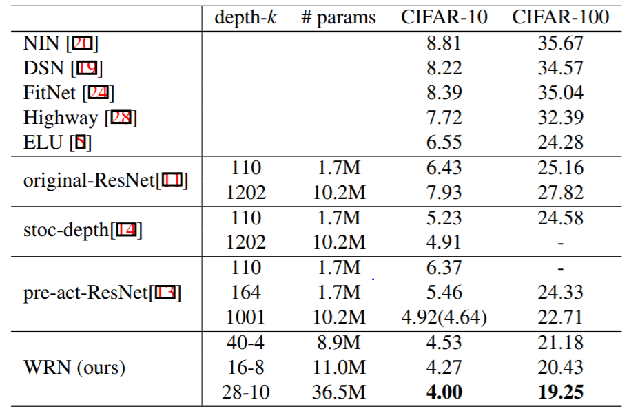
The following table compares the complexity and performance of Wide ResNet with several other models, including the original ResNet, on both CIFAR-10 and CIFAR-100:

Below are a few important links for implementing Wide ResNet yourself:

1. Link to the Original Paper
2. PyTorch Implementation of Wide ResNet
3. Tensorflow Implementation of Wide ResNet

Inception v3 (2015)

Inception v3 mainly focuses on burning less computational power by modifying the previous Inception architectures. This idea was proposed in the paper Rethinking the Inception Architecture for Computer Vision, published in 2015. It was co-authored by Christian Szegedy, Vincent Vanhoucke, Sergey Ioffe, and Jonathon Shlens.

In comparison to VGGNet, Inception Networks (GoogLeNet/Inception v1) have proved to be more computationally efficient, both in terms of the number of parameters generated by the network and the economical cost incurred (memory and other resources). If any changes are to be made to an Inception Network, care needs to be taken to make sure that the computational advantages aren’t lost. Thus, the adaptation of an Inception network for different use cases turns out to be a problem due to the uncertainty of the new network’s efficiency. In an Inception v3 model, several techniques for optimizing the network have been put suggested to loosen the constraints for easier model adaptation. The techniques include factorized convolutions, regularization, dimension reduction, and parallelized computations.

Inception v3 Architecture

The architecture of an Inception v3 network is progressively built, step-by-step, as explained below:

1. Factorized Convolutions: this helps to reduce the computational efficiency as it reduces the number of parameters involved in a network. It also keeps a check on the network efficiency.

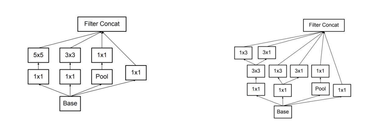
2. Smaller convolutions: replacing bigger convolutions with smaller convolutions definitely leads to faster training. Say a 5 × 5 filter has 25 parameters; two 3 × 3 filters replacing a 5 × 5 convolution has only 18 (3*3 + 3*3) parameters instead.

3. Asymmetric convolutions: A 3 × 3 convolution could be replaced by a 1 × 3 convolution followed by a 3 × 1 convolution. If a 3 × 3 convolution is replaced by a 2 × 2 convolution, the number of parameters would be slightly higher than the asymmetric convolution proposed.

4. Auxiliary classifier: an auxiliary classifier is a small CNN inserted between layers during training, and the loss incurred is added to the main network loss. In GoogLeNet auxiliary classifiers were used for a deeper network, whereas in Inception v3 an auxiliary classifier acts as a regularizer.

5. Grid size reduction: Grid size reduction is usually done by pooling operations. However, to combat the bottlenecks of computational cost, a more efficient technique is proposed:

All the above concepts are consolidated into the final architecture.

Inception v3 Training and Results

Inception v3 was trained on ImageNet and compared with other contemporary models, as shown below.

As shown in the table, when augmented with an auxiliary classifier, factorization of convolutions, RMSProp, and Label Smoothing, Inception v3 can achieve the lowest error rates compared to its contemporaries.

Below are a few relevant links if you're looking to implement Inception v3 yourself:

1. Link to the Original Research Paper
2. TensorFlow Implementation of Inception v3
3. PyTorch Implementation of Inception v3

SqueezeNet (2016)

SqueezeNet is a smaller network that was designed as a more compact replacement for AlexNet. It has almost 50x fewer parameters than AlexNet, yet it performs 3x faster. This architecture was proposed by researchers at DeepScale, The University of California, Berkeley, and Stanford University in the year 2016. It was first published in their paper titled SqueezeNet: AlexNet-level accuracy with 50x fewer parameters and <0.5MB model size.

Below are the key ideas behind SqueezeNet:

• Strategy One: use 1 × 1 filters instead of 3 × 3
• Strategy Two: decrease the number of input channels to 3 × 3 filters
• Strategy Three: Downsample late in the network so that convolution layers have large activation maps

SqueezeNet Architecture and Results

The SqueezeNet architecture is comprised of "squeeze" and "expand" layers. A squeeze convolutional layer has only 1 × 1 filters. These are fed into an expand layer that has a mix of 1 × 1 and 3 × 3 convolution filters. This is shown below.

The authors of the paper use the term “fire module”  to describe a squeeze layer and an expand layer together.

An input image is first sent into a standalone convolutional layer. This layer is followed by 8 "fire modules" which are named “fire2-9”, according to Strategy One above. The illustration of the resulting SqueezeNet is shown below.

Following Strategy Two, the filters per fire module are increased with "simple bypass." Lastly, SqueezeNet performs max-pooling with a stride of 2 after layers conv1, fire4, fire8, and conv10. According to Strategy Three, pooling is given a relatively late placement, resulting in SqueezeNet with a "complex bypass" (the rightmost architecture in the image above)

Below is an image showing how SqueezeNet compares with the original AlexNet.

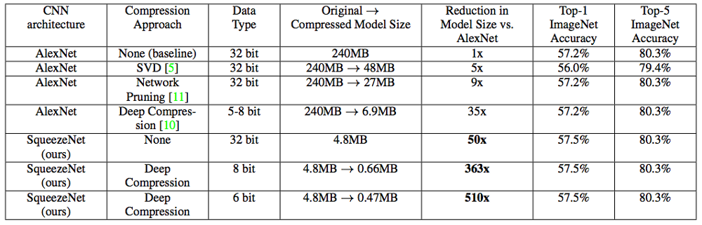
As we can observe, the weights of the compressed model for AlexNet were 240MB and achieved 80.3% accuracy. Meanwhile, a Deep Compression SqueezeNet consumes 0.47MB of memory and achieves the same performance.

Below are the details of other parameters used in the network:

• The ReLU activation is applied between all the squeeze and expand layers inside the fire module.
• Dropout layers are added to reduce overfitting, with a probability of 0.5 after the fire9 module.
• There are no fully connected layers used in the network. This design choice was inspired by the Network In Netowork (NIN) architecture proposed by (Lin et al, 2013).
• SqueezeNet was trained with a learning rate of 0.04, which is linearly decreased throughout the training process.
• The batch size for training is 32, and the network used an Adam Optimizer.

SqueezeNet makes the deployment process easier due to its small size. Initially this network was implemented in Caffe, but the model has since gained in popularity and has been adopted to many different platforms.

Below are a few relevant links for implementing SqueezeNet on your own, or further investigating the original implementation:

1. Link to the Original Implementation of SqueezeNet
2. Link to the Research Paper
3. SqueezeNet in Tensorflow
4. SqueezeNet in PyTorch

In third and final part of this series we'll cover the most recently-published models from 2017 to 2019: DenseNet, ResNeXt, MnasNet, and ShuffleNet v2.