Bring this project to life
When it comes to deep learning, most frameworks do not come with prepackaged training, validation and accuracy functions or methods. Getting started with these functionalities can therefore be a challenge to many engineers when they are first tackling data science problems. In most cases, these processes need to be manually implemented. At this point, it becomes tricky. In order to write these functions, one needs to actually understand what the processes entail. In this beginner's tutorial article, we will examine the above mentioned processes theoretically at a high level and implement them in PyTorch before putting them together and training a convolutional neural network for a classification task.
Imports and setup
Below are some of the imported libraries we will use for the task. Each is pre-installed in Gradient Notebook's Deep Learning runtimes, so use the link above to quick start this tutorial on a free GPU.
import torch
import torch.nn as nn
import torch.nn.functional as F
import torchvision
import torchvision.transforms as transforms
import torchvision.datasets as Datasets
from torch.utils.data import Dataset, DataLoader
import numpy as np
import matplotlib.pyplot as plt
import cv2
from tqdm.notebook import tqdm
if torch.cuda.is_available():
device = torch.device('cuda:0')
print('Running on the GPU')
else:
device = torch.device('cpu')
print('Running on the CPU')Anatomy of Neural Networks
Firstly, when talking about a model borne from a neural network, be it a multi layer perceptron, convolutional neural network or generative adversarial network etc, these models are simply made up of 'numbers', numbers which are weights and biases collectively called parameters. A neural network with 20 million parameters is simply one with 20 million numbers, each one influencing any instance of data that passes through the network (multiplicative for weights, additive for biases). Following this logic, when a 28 x 28 pixel image is passed through a convolutional neural network with 20 million parameters, all 784 pixels will in fact encounter and be transformed by all 20 million parameters in some way.
Model Objective
Consider the custom built convnet below, the output layer returns a two element vector representation therefore it is safe to conclude that its objective is to help solve a binary classification task.
class ConvNet(nn.Module):
  def __init__(self):
    super().__init__()
    self.conv1 = nn.Conv2d(3, 8, 3, padding=1)
    self.batchnorm1 = nn.BatchNorm2d(8)
    self.conv2 = nn.Conv2d(8, 8, 3, padding=1)
    self.batchnorm2 = nn.BatchNorm2d(8)
    self.pool2 = nn.MaxPool2d(2)
    self.conv3 = nn.Conv2d(8, 32, 3, padding=1)
    self.batchnorm3 = nn.BatchNorm2d(32)
    self.conv4 = nn.Conv2d(32, 32, 3, padding=1)
    self.batchnorm4 = nn.BatchNorm2d(32)
    self.pool4 = nn.MaxPool2d(2)
    self.conv5 = nn.Conv2d(32, 128, 3, padding=1)
    self.batchnorm5 = nn.BatchNorm2d(128)
    self.conv6 = nn.Conv2d(128, 128, 3, padding=1)
    self.batchnorm6 = nn.BatchNorm2d(128)
    self.pool6 = nn.MaxPool2d(2)
    self.conv7 = nn.Conv2d(128, 2, 1)
    self.pool7 = nn.AvgPool2d(3)

  def forward(self, x):
    #-------------
    # INPUT
    #-------------
    x = x.view(-1, 3, 32, 32)

    #-------------
    # LAYER 1
    #-------------
    output_1 = self.conv1(x)
    output_1 = F.relu(output_1)
    output_1 = self.batchnorm1(output_1)

    #-------------
    # LAYER 2
    #-------------
    output_2 = self.conv2(output_1)
    output_2 = F.relu(output_2)
    output_2 = self.pool2(output_2)
    output_2 = self.batchnorm2(output_2)

    #-------------
    # LAYER 3
    #-------------
    output_3 = self.conv3(output_2)
    output_3 = F.relu(output_3)
    output_3 = self.batchnorm3(output_3)

    #-------------
    # LAYER 4
    #-------------
    output_4 = self.conv4(output_3)
    output_4 = F.relu(output_4)
    output_4 = self.pool4(output_4)
    output_4 = self.batchnorm4(output_4)

    #-------------
    # LAYER 5
    #-------------
    output_5 = self.conv5(output_4)
    output_5 = F.relu(output_5)
    output_5 = self.batchnorm5(output_5)

    #-------------
    # LAYER 6
    #-------------
    output_6 = self.conv6(output_5)
    output_6 = F.relu(output_6)
    output_6 = self.pool6(output_6)
    output_6 = self.batchnorm6(output_6)

    #--------------
    # OUTPUT LAYER
    #--------------
    output_7 = self.conv7(output_6)
    output_7 = self.pool7(output_7)
    output_7 = output_7.view(-1, 2)

    return F.softmax(output_7, dim=1)
Assume we would like to train this convnet to correctly distinguish cats, labelled 0, from dogs, labelled 1. Essentially, what we are trying to do on a low level is to ensure that whenever an image of a cat is passed through the network, and all it's pixels interact with all 197,898 parameters in this convnet, that the first element in the output vector (index 0) will be greater than the second element (index 1) {eg [0.65, 0.35]}. Otherwise, if an image of a dog is passed through, then the second element (index 1) is expected to be greater {eg [0.20, 0.80]}.
Now, we can begin to perceive the enormity of the model objective, and, yes, there exist a combination of 197,898 numbers/parameters in the millions of permutations possible that allow us to do just that which we have described in the previous paragraph. Looking for this permutation is simply what the training process entails.
The Right Combination
When ever a neural network is instantiated, it's parameters are all randomized, or if you are initializing parameters through a particular technique they will not be random but follow initializations specific to that particular technique. Notwithstanding, at initialization the network parameters will not fit the model objective at hand such that if the model is used in that state random classifications will be obtained.
The goal now is to find the right combination of 197,898 parameters which will allow us to archive our objective. To do this, we need to break training images into batches, and then pass a batch through the convnet, measure how wrong our classifications are (forward propagation), adjust all 197,898 parameters slightly in the direction which best fits our objective (backpropagation), and then repeat for all other batches until the training data is exhausted. This process is called optimization.
def train(network, training_set, batch_size, optimizer, loss_function):
  """
  This function optimizes the convnet weights
  """
  #  creating list to hold loss per batch
  loss_per_batch = []

  #  defining dataloader
  train_loader = DataLoader(training_set, batch_size)

  #  iterating through batches
  print('training...')
  for images, labels in tqdm(train_loader):
    #---------------------------
    #  sending images to device
    #---------------------------
    images, labels = images.to(device), labels.to(device)

    #-----------------------------
    #  zeroing optimizer gradients
    #-----------------------------
    optimizer.zero_grad()

    #-----------------------
    #  classifying instances
    #-----------------------
    classifications = network(images)

    #---------------------------------------------------
    #  computing loss/how wrong our classifications are
    #---------------------------------------------------
    loss = loss_function(classifications, labels)
    loss_per_batch.append(loss.item())

    #------------------------------------------------------------
    #  computing gradients/the direction that fits our objective
    #------------------------------------------------------------
    loss.backward()

    #---------------------------------------------------
    #  optimizing weights/slightly adjusting parameters
    #---------------------------------------------------
    optimizer.step()
  print('all done!')

  return loss_per_batch
Proper Generalization
In order to ensure that the optimized parameters work on data outside the training set, we need to utilize them in classifying a different set of images and ensure that they have comparable performance as they did on the training set, this time no optimization will be done on the parameters. This process is called validation, and the dataset used for this purpose is called the validation set.
def validate(network, validation_set, batch_size, loss_function):
  """
  This function validates convnet parameter optimizations
  """
  #  creating a list to hold loss per batch
  loss_per_batch = []

  #  defining model state
  network.eval()

  #  defining dataloader
  val_loader = DataLoader(validation_set, batch_size)

  print('validating...')
  #  preventing gradient calculations since we will not be optimizing
  with torch.no_grad():
    #  iterating through batches
    for images, labels in tqdm(val_loader):
      #--------------------------------------
      #  sending images and labels to device
      #--------------------------------------
      images, labels = images.to(device), labels.to(device)

      #--------------------------
      #  making classsifications
      #--------------------------
      classifications = network(images)

      #-----------------
      #  computing loss
      #-----------------
      loss = loss_function(classifications, labels)
      loss_per_batch.append(loss.item())

  print('all done!')

  return loss_per_batch
Measuring Performance
While dealing with a classification task in the context of a balanced training set, model performance is best measured using accuracy as the metric of choice. Since labels are integers which are essentially pointers to the index which should have the highest probability/value, to derive accuracy we need to compare the index of the maximum value in the output vector representation when an image passes through the convnet with with the image's label. Accuracy is measured on both the training and validation set.
def accuracy(network, dataset):
  """
  This function computes accuracy
  """
  #  setting model state
  network.eval()

  #  instantiating counters
  total_correct = 0
  total_instances = 0

  #  creating dataloader
  dataloader = DataLoader(dataset, 64)

  #  iterating through batches
  with torch.no_grad():
    for images, labels in tqdm(dataloader):
      images, labels = images.to(device), labels.to(device)

      #-------------------------------------------------------------------------
      #  making classifications and deriving indices of maximum value via argmax
      #-------------------------------------------------------------------------
      classifications = torch.argmax(network(images), dim=1)

      #--------------------------------------------------
      #  comparing indicies of maximum values and labels
      #--------------------------------------------------
      correct_predictions = sum(classifications==labels).item()

      #------------------------
      #  incrementing counters
      #------------------------
      total_correct+=correct_predictions
      total_instances+=len(images)
  return round(total_correct/total_instances, 3)
Connecting the Pieces
Bring this project to life
Dataset
In order to observe all these processes working in synergy, we will now apply them on an actual dataset. The CIFAR-10 dataset will be used for this purpose. This is a dataset containing 32 x 32 pixel images from 10 different classes as outlined in the table below.
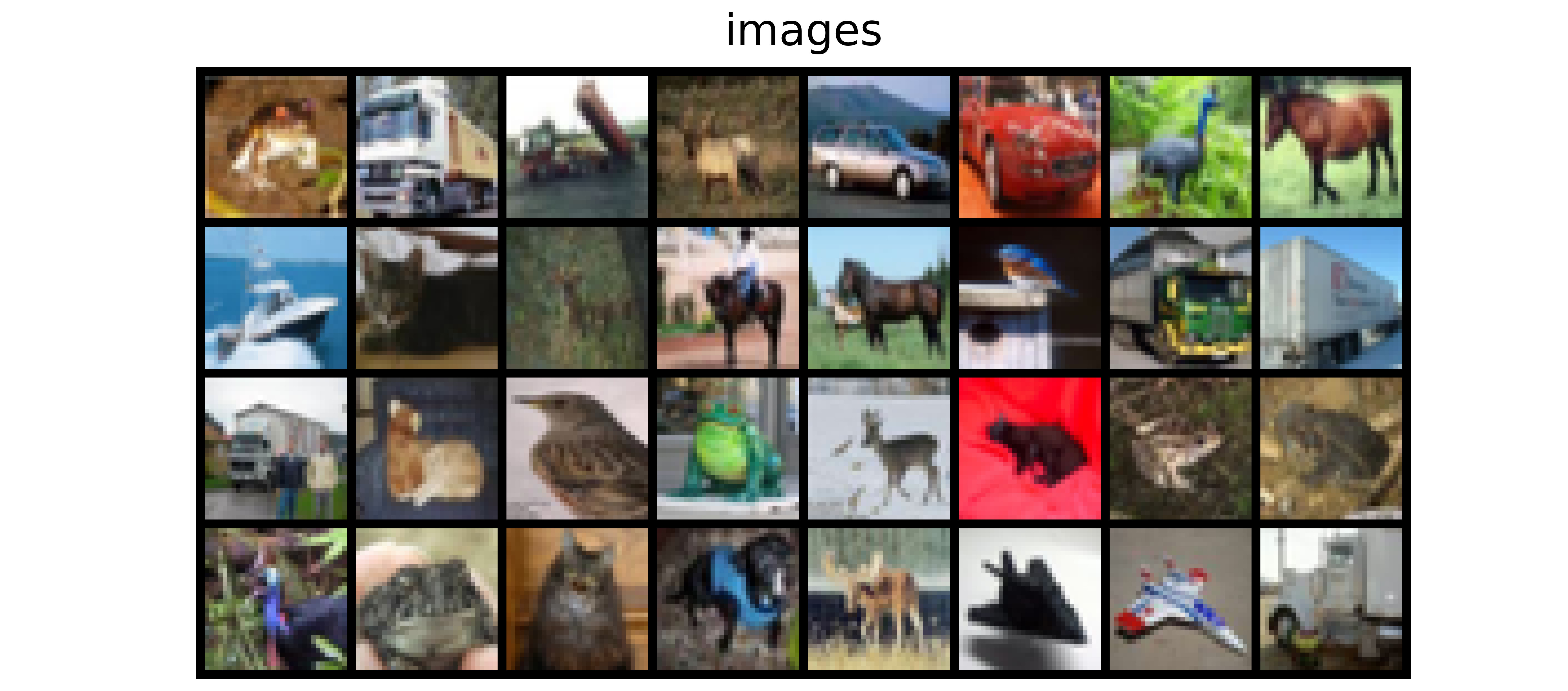
The dataset can be loaded in PyTorch as follows...
#  loading training data
training_set = Datasets.CIFAR10(root='./', download=True,
                              transform=transforms.ToTensor())

#  loading validation data
validation_set = Datasets.CIFAR10(root='./', download=True, train=False,
transform=transforms.ToTensor())| label | Description |
|---|---|
| 0 | airplane |
| 1 | automobile |
| 2 | bird |
| 3 | cat |
| 4 | deer |
| 5 | dog |
| 6 | frog |
| 7 | horse |
| 8 | ship |
| 9 | truck |
Convnet Architecture
Since this is a 10 class classification task, we need to modify our convnet to output a 10 element vector as done in the following code cell.
class ConvNet(nn.Module):
  def __init__(self):
    super().__init__()
    self.conv1 = nn.Conv2d(3, 8, 3, padding=1)
    self.batchnorm1 = nn.BatchNorm2d(8)
    self.conv2 = nn.Conv2d(8, 8, 3, padding=1)
    self.batchnorm2 = nn.BatchNorm2d(8)
    self.pool2 = nn.MaxPool2d(2)
    self.conv3 = nn.Conv2d(8, 32, 3, padding=1)
    self.batchnorm3 = nn.BatchNorm2d(32)
    self.conv4 = nn.Conv2d(32, 32, 3, padding=1)
    self.batchnorm4 = nn.BatchNorm2d(32)
    self.pool4 = nn.MaxPool2d(2)
    self.conv5 = nn.Conv2d(32, 128, 3, padding=1)
    self.batchnorm5 = nn.BatchNorm2d(128)
    self.conv6 = nn.Conv2d(128, 128, 3, padding=1)
    self.batchnorm6 = nn.BatchNorm2d(128)
    self.pool6 = nn.MaxPool2d(2)
    self.conv7 = nn.Conv2d(128, 10, 1)
    self.pool7 = nn.AvgPool2d(3)

  def forward(self, x):
    #-------------
    # INPUT
    #-------------
    x = x.view(-1, 3, 32, 32)

    #-------------
    # LAYER 1
    #-------------
    output_1 = self.conv1(x)
    output_1 = F.relu(output_1)
    output_1 = self.batchnorm1(output_1)

    #-------------
    # LAYER 2
    #-------------
    output_2 = self.conv2(output_1)
    output_2 = F.relu(output_2)
    output_2 = self.pool2(output_2)
    output_2 = self.batchnorm2(output_2)

    #-------------
    # LAYER 3
    #-------------
    output_3 = self.conv3(output_2)
    output_3 = F.relu(output_3)
    output_3 = self.batchnorm3(output_3)

    #-------------
    # LAYER 4
    #-------------
    output_4 = self.conv4(output_3)
    output_4 = F.relu(output_4)
    output_4 = self.pool4(output_4)
    output_4 = self.batchnorm4(output_4)

    #-------------
    # LAYER 5
    #-------------
    output_5 = self.conv5(output_4)
    output_5 = F.relu(output_5)
    output_5 = self.batchnorm5(output_5)

    #-------------
    # LAYER 6
    #-------------
    output_6 = self.conv6(output_5)
    output_6 = F.relu(output_6)
    output_6 = self.pool6(output_6)
    output_6 = self.batchnorm6(output_6)

    #--------------
    # OUTPUT LAYER
    #--------------
    output_7 = self.conv7(output_6)
    output_7 = self.pool7(output_7)
    output_7 = output_7.view(-1, 10)

    return F.softmax(output_7, dim=1)
Joining Processes
In order to train the above defined convnet, all we need to do is to instantiate the model, utilize the training function in optimizing the convnet weights, and record how wrong our classifications are on each batch (loss). We then utilize the validation function to ensure the convnet works on data outside the training set, and again record how wrong our classifications are. We then derive the convnets accuracy on the training and validation set, recording losses at each step to keep track of the optimization process.
#  instantiating model
model = ConvNet()
#  defining optimizer
optimizer = torch.optim.Adam(model.parameters(), lr=3e-4)

#  training/optimizing parameters
training_losses = train(network=model, training_set=training_set,
                        batch_size=64, optimizer=optimizer,
                        loss_function=nn.CrossEntropyLoss())

#  validating optimizations
validation_losses = validate(network=model, validation_set=validation_set,
                             batch_size=64, loss_function=nn.CrossEntropyLoss())

#  deriving model accuracy on the traininig set
training_accuracy = accuracy(model, training_set)
print(f'training accuracy: {training_accuracy}')

#  deriving model accuracy on the validation set
validation_accuracy = accuracy(model, validation_set)
print(f'validation accuracy: {validation_accuracy}')
There's a good chance that when you run the code block above your training and validation accuracies will be less than ideal. However, if you take the first four lines of code out and paste them in a new code cell, rerunning the training, validation and accuracy functions will yield an increase in performance. This process of taking numerous cycles through the whole dataset is known as training for epochs. Essentially, if you run the processes five time you've trained the model for 5 epochs.
The reason for moving the first four lines of code is that at the point of running the training function, the randomly initialized weights in the model have been optimized to a point. If you then rerun the code cell with your model instantiation still in the same cell, then its weights will be randomized once again and render the previous optimization null. In a bid to make sure all processes are properly synchronized, it is a good idea to package than in a function or a class. I personally prefer using classes as it keeps all processes in a neat package.
class ConvolutionalNeuralNet():
  def __init__(self, network):
    self.network = network.to(device)
    self.optimizer = torch.optim.Adam(self.network.parameters(), lr=1e-3)

  def train(self, loss_function, epochs, batch_size,
            training_set, validation_set):

    #  creating log
    log_dict = {
        'training_loss_per_batch': [],
        'validation_loss_per_batch': [],
        'training_accuracy_per_epoch': [],
        'validation_accuracy_per_epoch': []
    }

    #  defining weight initialization function
    def init_weights(module):
      if isinstance(module, nn.Conv2d):
        torch.nn.init.xavier_uniform_(module.weight)
        module.bias.data.fill_(0.01)
      elif isinstance(module, nn.Linear):
        torch.nn.init.xavier_uniform_(module.weight)
        module.bias.data.fill_(0.01)

    #  defining accuracy function
    def accuracy(network, dataloader):
      network.eval()
      total_correct = 0
      total_instances = 0
      for images, labels in tqdm(dataloader):
        images, labels = images.to(device), labels.to(device)
        predictions = torch.argmax(network(images), dim=1)
        correct_predictions = sum(predictions==labels).item()
        total_correct+=correct_predictions
        total_instances+=len(images)
      return round(total_correct/total_instances, 3)

    #  initializing network weights
    self.network.apply(init_weights)

    #  creating dataloaders
    train_loader = DataLoader(training_set, batch_size)
    val_loader = DataLoader(validation_set, batch_size)

    #  setting convnet to training mode
    self.network.train()

    for epoch in range(epochs):
      print(f'Epoch {epoch+1}/{epochs}')
      train_losses = []

      #  training
      print('training...')
      for images, labels in tqdm(train_loader):
        #  sending data to device
        images, labels = images.to(device), labels.to(device)
        #  resetting gradients
        self.optimizer.zero_grad()
        #  making predictions
        predictions = self.network(images)
        #  computing loss
        loss = loss_function(predictions, labels)
        log_dict['training_loss_per_batch'].append(loss.item())
        train_losses.append(loss.item())
        #  computing gradients
        loss.backward()
        #  updating weights
        self.optimizer.step()
      with torch.no_grad():
        print('deriving training accuracy...')
        #  computing training accuracy
        train_accuracy = accuracy(self.network, train_loader)
        log_dict['training_accuracy_per_epoch'].append(train_accuracy)

      #  validation
      print('validating...')
      val_losses = []

      #  setting convnet to evaluation mode
      self.network.eval()

      with torch.no_grad():
        for images, labels in tqdm(val_loader):
          #  sending data to device
          images, labels = images.to(device), labels.to(device)
          #  making predictions
          predictions = self.network(images)
          #  computing loss
          val_loss = loss_function(predictions, labels)
          log_dict['validation_loss_per_batch'].append(val_loss.item())
          val_losses.append(val_loss.item())
        #  computing accuracy
        print('deriving validation accuracy...')
        val_accuracy = accuracy(self.network, val_loader)
        log_dict['validation_accuracy_per_epoch'].append(val_accuracy)

      train_losses = np.array(train_losses).mean()
      val_losses = np.array(val_losses).mean()

      print(f'training_loss: {round(train_losses, 4)}  training_accuracy: '+
      f'{train_accuracy}  validation_loss: {round(val_losses, 4)} '+
      f'validation_accuracy: {val_accuracy}\n')

    return log_dict

  def predict(self, x):
    return self.network(x)
In the class above, we have combined both the training and validation processes in the train() method. This is to prevent making multiple attribute calls as these processes work in tandem anyway. Also notice that accuracy is added as a helper function within the train() method and accuracy is computed immediately after training and validation. A weight initialization function which helps to initialize weights using the Xavier weight initialization technique is also defined, it is typically good practice to have a degree of control over how a network's weights are initialized. A metric log is also defined to keep track of all losses and accuracies as the convnet is trained.
# training model
model = ConvolutionalNeuralNet(ConvNet())
log_dict = model.train(nn.CrossEntropyLoss(), epochs=10, batch_size=64,
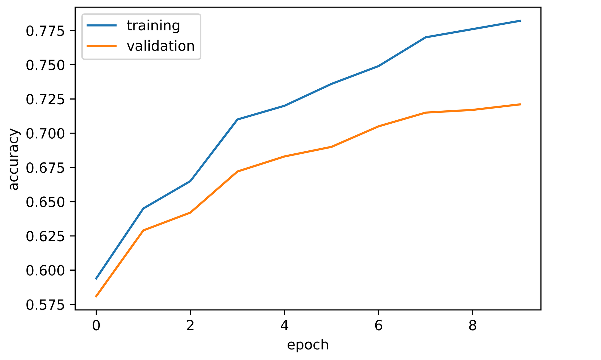
training_set=training_set, validation_set=validation_set)Training the convnet for 10 epochs (10 cycles) with the above defined parameters yielded the metrics below. Both training and validation accuracy increased through the course of training which indicates that the convnets parameters were indeed being adjusted/optimized properly. Validation accuracy started off at about 58% and was able to reach 72% by the tenth epoch.
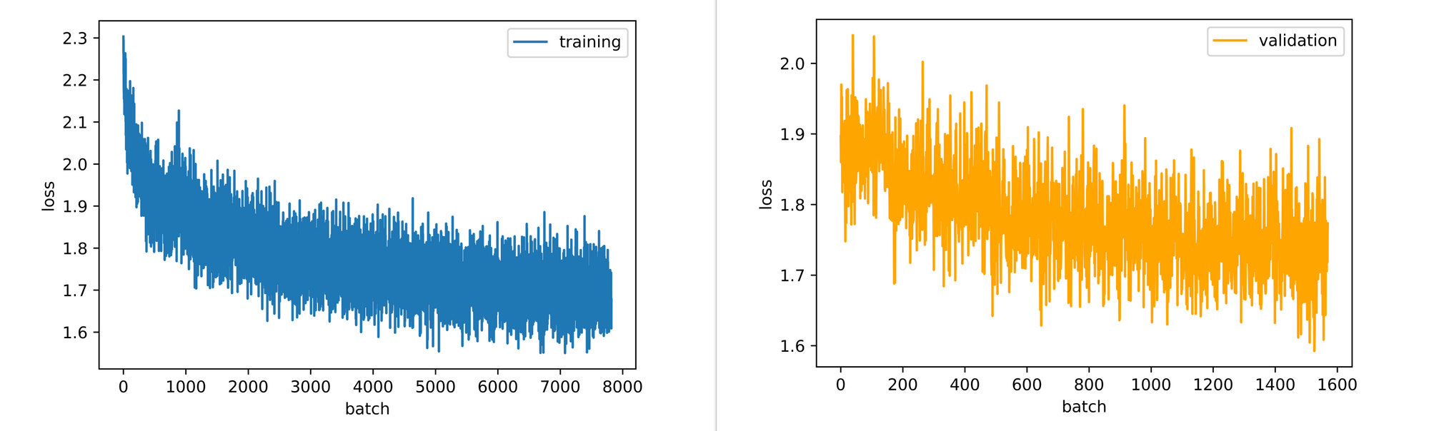
It should be noted however that the convnet wasn't trained exhaustively as even though the validation curve had began to flatten, it is still on an upward trend so the convnet could probably take a few more epochs of training before overfitting comes into play. The loss plots also point to the same situation as validation loss per batch is still down-trending at the end of the 10th epoch.
Final Remarks
In this article we explored three vital processes in the training of neural networks: training, validation and accuracy. We explained at a high level what all three processes entail and how they can be implemented in PyTorch. We then combined all three processes in a class and used it in training a convolutional neural network. Readers should expect to be able to implement these functionalities in their own PyTorch code going forward.