
Bring this project to life
Upon developing an intuition for convolutional neural network processes such as convolution, padding and pooling, the natural next step is to then put them all together in such a way that they work in tandem to archive a particular objective. When all of these processes are put together an architecture is produced.
The configuration of an architecture determines to a large extent how well a certain network will perform. In this article, we will be taking a look at CNN architectures with a view at understanding what happens to an image as it passes from one layer to the other in terms of spatial dimension up until the output layer.
Notation Used In This Article
The default notation for specifying the dimension of matrices/arrays is to start specifications from the number of rows (height), to the number of columns (width), then number of channels and finally, batch size. Following this notation, 15 matrices of size 250 x 320 pixels and 3 channels would be specified (250, 320, 3, 15).
However, in this article, we will be using the PyTorch notation which begins specification from batch size, to number of channels, then number of rows and finally, number of columns. Using this notation, the matrices in the paragraph above will be specified as (15, 3, 250, 320) . Please bare this in mind.
Convolution Over Channels
In a previous article, I mentioned how the convolution process is used to extract features from images. For illustration purposes, I had used a single channel image (grayscale), that is, an image made up of a single array of pixels. In most cases, in fact in all cases as regards convolutional neural networks, the convolution operation is applied to an image or set of feature maps with more than one channel.
Consider a case where one intends to perform convolution on a colored image. As we all know, colored images have 3 RGB channels (3 arrays), in order to produce a single feature map from this image (detect edges for instance), one needs a filter which has a corresponding number of channels.
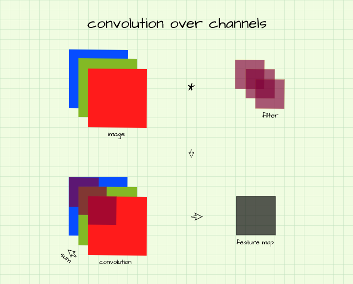
In essence, this means there will be one convolution filter for every channel in the image, with the result of corresponding convolution instances summed up across channels to produce a single pixel in the feature map. In more technical terms, in order to produce a single feature map a (3, 6, 6) (3 channels, 6 rows, 6 columns) image is convolved using a (3, 3, 3) (3 channels, 3 rows, 3 columns) filter. Following the same logic, if one intends to produce 10 feature maps from that image then 10 (3, 3, 3) filters are required, i.e (10, 3, 3, 3).
Sliding Window Operations & Feature Map Dimensions
Sliding window operations such as convolution and pooling make up the vast majority of operations in convolutional neural networks. It is worth remembering that these sliding window operations often modify the dimensions of images/feature maps. Some of these modifications are deliberate while others are a by-product with padding used to control what happens with the representation produced.
Just as I mentioned in this article, I'll paraphrase, if a filter/kernel of size (m, n) is slid over an image of size (x, y), then a representation of size (x-m+1, y-n+1) is produced. Now when strides greater than one and padding are involved in these operation, this formula can be rewritten as:
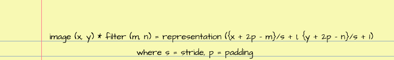
Therefore, if a (3, 3) filter is slid over a (55, 55) image using a stride of 2, a representation of size (27, 27) (({55-3}/2 + 1 , {55-3}/2 + 1)) is produced.
Activation Functions
Activation functions are a common sight in neural network architectures as they play a vital role in network performance. They serve the purpose of adding non-linearity to the network itself as they force the network to learn a more complex mapping/relationship between inputs and outputs (more on this in a coming article).
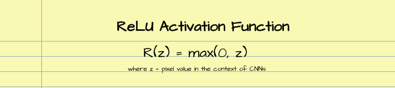
In the context of convolutional neural network architectures, the Rectified Linear Unit activation function, ReLU, or some other variation of it (Parametric ReLU, Leaky-ReLU) is most commonly used. This activation function essentially looks through the pixels in feature maps and leaves them untouched if they have a value greater than zero or sets them to zero if they have a value less than zero (negative value). In more simple terms, the ReLU activation function switches off less essential pixels in a feature map.
Regularization In Convolutional Neural Networks
Regularization refers to techniques used in machine learning to prevent a model from over-fitting. In the deep learning, the two main regularization techniques are termed batch normalization and dropout.
Batch normalization works by normalizing all inputs in the layer in which it is used, it has the unique advantage of preventing internal covariate shift in neural networks and speeding up model training. Some studies have deemed it most suitable for convolution layers.
On the other hand, dropout works by randomly zeroing certain neurons in the layer in which it is applied, by doing this it simulates a slightly different network architecture for each batch of data during training thereby preventing the native network from over-fitting data. There are some literature to suggest that it works best on linear layers.
Sections In Neural Network Architectures
A neural network is made up of layers. These layers can be grouped into 3 sections such as the input layer, hidden layers and the output layer.
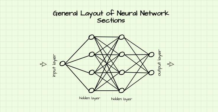
As the name suggests, the input layer is the portion of the neural network is where data is fed through. On the other hand, the hidden layers are the layers in the network which sit between the input and output layers. This portion of the network (hidden layers) is responsible for computation and numerical transformation of data while the output layer is the final layer of the network where a result/output is obtained.
The AlexNet Architecture
AlexNet is a convolutional neural network architecture designed by Alex Krizhevsky, Ilya Sutskever and Geoffery Hinton in 2012 (Krizhevsky et al, 2012). Although a bit dated at the moment, this architecture was quite ground breaking at the time as it helped to form the basis of common convolutional neural network best practices such as the predominant use of the ReLU non-linearity as well as an assertion that network performance improves with an increase in depth. It is also quite simple enough to easy grasp and interpret.
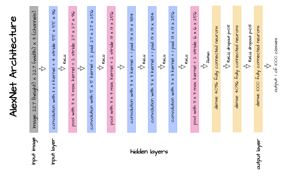
Using the pictorial representation of the AlexNet architecture as seen above, let's attempt to replicate this architecture using PyTorch. Thereafter, we will perform a walk-through of each layer so as to understand how an image goes from raw pixels in the input layer to feature maps in the hidden layers and finally a classification vector in the output layer.
Bring this project to life
class AlexNet(nn.Module):
    def __init__(self):
      super().__init__()
      #  instantiating network classes
      self.conv1 = nn.Conv2d(3, 96, (11, 11), stride=4)
      self.pool1 = nn.MaxPool2d((3, 3), stride=2)
      self.conv2 = nn.Conv2d(96, 256, (5, 5), padding=2)
      self.pool2 = nn.MaxPool2d((3, 3), stride=2)
      self.conv3 = nn.Conv2d(256, 384, (3, 3), padding=1)
      self.conv4 = nn.Conv2d(384, 384, (3, 3), padding=1)
      self.conv5 = nn.Conv2d(384, 256, (3, 3), padding=1)
      self.pool5 = nn.MaxPool2d((3, 3), stride=2)
      self.dense1 = nn.Linear(9216, 4096)
      self.dense2 = nn.Linear(4096, 4096)
      self.dense3 = nn.Linear(4096, 1000)
      self.dropout = nn.Dropout(p=0.5)

    def forward(self, x):
      #-------------------
      #  INPUT IMAGE(S)
      #-------------------
      input = x.view(-1, 3, 227, 227) # -> (3, 227, 227)

      #-------------------
      #  INPUT LAYER
      #-------------------
      #  convolution -> activation -> pooling
      layer_1 = self.conv1(x) # -> (96, 55, 55)
      output_1 = F.relu(layer_1)
      output_1 = self.pool1(output_1) # -> (96, 27, 27)

      #-------------------
      #  HIDDEN LAYERS
      #-------------------
      #  convolution -> activation -> pooling
      layer_2 = self.conv2(output_1) # -> (256, 27, 27)
      output_2 = F.relu(layer_2)
      output_2 = self.pool2(output_2) # -> (256, 13, 13)

      #  convolution -> activation
      layer_3 = self.conv3(output_2) # -> (384, 13, 13)
      output_3 = F.relu(layer_3)

      #  convolution -> activation
      layer_4 = self.conv4(output_3) # -> (384, 13, 13)
      output_4 = F.relu(layer_4)

      #  convolution -> activation -> pooling
      layer_5 = self.conv5(output_4) # -> (256, 13, 13)
      output_5 = F.relu(layer_5)
      output_5 = self.pool5(output_5) # -> (256, 6, 6)

      #  flattening feature map
      flattened = output_5.view(-1, 9216) # (256*6*6 = 9216)

      #  full connection -> activation -> dropout
      layer_6 = self.dense1(flattened) # -> (1, 4096)
      output_6 = F.relu(layer_6)
      output_6 = self.dropout(output_6)

      #  full connection -> activation -> dropout
      layer_7 = self.dense2(layer_6) # -> (1, 4096)
      output_7 = F.relu(layer_7)
      output_7 = self.dropout(output_7)

      #--------------------
      # OUTPUT LAYER
      #--------------------
      layer_8 = self.dense3(layer_7) # -> (1, 1000)
      output_8 = torch.sigmoid(layer_8)
      return output_8
The architecture is implemented by firstly instantiating the required convolution, pooling, linear and dropout methods in the init method. Thereafter, the network is put together in the forward method. This implementation could also be done using the PyTorch sequential method but I decided against that as it could get quite cumbersome to explain. You might find that the above code is a bit comment heavy, this is to allow for easy understanding and explainability, a walk-through of all layers in the forward method is provided below.
Neural Network Methods Used
In this section, we will be taking a closer look at the neural network methods instantiated in the init method. Each method is aptly named so that it matches the layer in which it is used in the forward method.
self.conv1
This is a 2-dimensional convolution method which receives images or feature maps of 3 channels and produces 96 channels from them using (11, 11) filters with the filters taking a stride of 4 pixels after every instance.
self.pool1
This is a 2-dimensional max pooling method which utilizes a (3, 3) filter/kernel in effectively down-sampling feature maps by half their size as it utilizes a stride of 2. This is a case of overlapping pooling as the size of the kernel is not equal to its stride (3 != 2).
self.conv2
This is a 2-dimensional convolution method which receives feature maps of 96 channels and produces 256 channels from them using (5, 5) filters with a default stride of 1 and 2 layers of padding implying that the channels produced will not be of reduced dimensions.
self.pool2
Just like self.pool1, this is a 2-dimensional max pooling method which utilizes a (3, 3) filter/kernel in effectively down-sampling feature maps by half their size as it utilizes a stride of 2.
self.conv3
This is a 2-dimensional convolution method which receives feature maps of 256 channels and produces 384 channels from them using (3, 3) filters with a default stride of 1 and a single padding layer implying that the channels produced will not be of reduced dimensions.
self.conv4
This is a 2-dimensional convolution method which receives feature maps of 384 channels and again produces 384 channels from them using (3, 3) filters with a default stride of 1 and a single padding layer implying that the representations produced will not reduce in dimension.
self.conv5
Seemingly the inverse of self.conv3, self.conv5 is a 2-dimensional convolution method which receives feature maps of 384 channels and produces 256 channels from them using (3, 3) filters with a default stride of 1 and a single padding layer implying that the channels produced will not be of reduced dimensions.
self.pool5
Just like self.pool1 and 2, this is a 2-dimensional max pooling method which utilizes a (3, 3) filter/kernel in effectively down-sampling feature maps by half their size as it utilizes a stride of 2.
self.dense1
This is a linear method which receives a vector of 9216 elements (size (1, 9216)) and connects them to another vector of 4096 elements (size (1, 4096)).
self.dense2
This is a linear method which receives a vector of 4096 elements (size (1, 4096)) and connects them to another vector of 4096 elements (size (1, 4096)).
self.dense3
This is a linear method which receives a vector of 4096 elements (size (1, 4096)) and connects them to another vector of 1000 elements (size (1, 1000)).
self.dropout
This is a dropout regularization method used to control over-fitting by choosing to ignore the output of randomly selected neurons with a 50% probability.
Input Image(s)
The parameter 'x' in the forward method is termed the input image. This is the image or batch of images passed to the network for classification purposes. Since the AlexNet architecture specifies a colored input image of size 227 pixels x 227 pixels, (3, 227, 227) , the input is viewed as a tensor of size (-1, 3, 227, 227). The first dimension accounts for the batch size and is specified as -1 so as to allow the network to accept any batch size (typically multiples of 8 during training and as little as 1 in production).
Input Layer
In layer 1, since we are trying to produce 96 feature maps using (11, 11) filters, a single input image of size (3, 227, 227) is convolved upon by 96 filters of size (3, 11, 11) with stride=4 so as to produce feature maps of size (96, 55, 55) . The size of the image reduces from (227, 227) to (55, 55)as evident from the formula ({x + 2p - m}/s + 1, {y + 2p - n}/s + 1). Note that padding is left as a default value of 0 so p=0 in this case.
Next, the feature maps produced are activated using the ReLU non-linearity and max pooled using (3, 3) kernels and stride=2 to down-sample them to (96, 27, 27). The feature maps become 27 x 27 pixels because overlapping pooling with a (3, 3) kernel and a stride of 2 was used. Again, remember ({x + 2p - m}/s + 1, {y + 2p - n}/s + 1).
Layer 2
In layer 2, 256 feature maps are to be produced from the feature maps from layer 1 (size (96, 27, 27)) using (5, 5) filters. To do that, 256 filters of size (96, 5, 5) are used. Since padding is set to 2, the feature maps produced do not reduce in size and are returned as (256, 27, 27). Thereafter, activation is done followed by pooling with a (3, 3) filter and stride=2 producing a feature map of size (256, 13, 13).
Layer 3
In layer 3, 386 feature maps are to be produced from the output of layer 2 (size (256, 13, 13)) using a (3, 3) filter. To do that, 386 filters of size (256, 5, 5) are used. Since padding is set to one, the feature maps produced remain the same size. Activation follows without pooling.
Layer 4
As regards layer 4, 386 feature maps are to be produced from the output of layer 3 (size (386, 13, 13)) using a (3, 3) filter. To do that, 386 filters of size (386, 5, 5) are used. Since padding is set to one, the feature maps produced remain the same size. Again, pooling is not done after activation as specified in the network architecture.
Layer 5
Layer 5 looks to be the reverse of layer 3 as 256 feature maps are to be produced from the output of layer 4 (size (386, 13, 13)) using a (3, 3) filter. To do that, 256 filters of size (386, 5, 5) are used. Since padding is set to one, the feature maps produced remain the same size. Pooling is done after activation to down-sample the feature maps to (256, 6, 6).
Layer 6
Right before layer 6, the feature maps are flattened since they are about to be fed into a dense layer which only accepts a vector. To flatten the feature maps, all of the dimensions of the feature maps returned as output from layer 5 are multiplied (256*6*6 = 9216) and reshaped into a vector (size (1, 9216)). This vector is then fed into layer 6 to produce another vector of 4096 elements (size (1, 4096)). The resulting vector is then activated with dropout applied thereafter.
Layer 7
The 4096 element vector returned as output from layer 6 are fed into this layer which again produces another vector of the same number of elements. ReLU activation follows before dropout is again applied.
Output Layer
Layer 8, also known as the output layer, receives the 4096 element vector form layer 7 and produces a 1000 element vector (size (1, 1000)) as final output. A 1000 element vector is produced as final output since the AlexNet architecture was used on the ImageNet dataset which contains 1000 classes. A sigmoid activation is then applied to the final output so as to return probabilities.
Parameters In a Convolutional Neural Network
Parameters in a neural network are the biases and weights which connect neurons from one layer to the other. This definition is more suitable for parameters in a linear layers, for parameters in convolutional layers, parameters can be said to be the total number of elements in the filters (these are the weights) contained in convolution layers and their biases.
It is a common thing to determine the number of parameters present in a certain neural network architecture. For instance, a single convolutional layer with 3 filters each with 3 channels and size (3, 3) has a total of 3 biases (one for each filter) and 81 weights (3*3*3*3), resulting in a total of 84 parameters.
Using this knowledge, let's try to determine the number of parameters present tin the AlexNet architecture above.
| Layers | Weights | Biases | Parameters |
|---|---|---|---|
| layer 1 | 11x11x3x96 = 34,848 | 96 | 34,944 |
| layer 2 | 5x5x96x256 = 614,400 | 256 | 614,656 |
| layer 3 | 3x3x256x384 = 884,736 | 384 | 885,120 |
| layer 4 | 3x3x384x384 = 1,327,104 | 384 | 1,327,488 |
| layer 5 | 3x3x384x256 = 884,736 | 256 | 884,992 |
| layer 6 | 9216x4096 = 37,748,736 | 4096 | 37,752,832 |
| layer 7 | 4096x4096 = 16,777,216 | 4096 | 16,781,312 |
| layer 8 | 4096x1000 = 4,096,000 | 1000 | 4,097,000 |
| Total | 62,378,344 |
From the table above, the AlexNet architecture has a total of about 62 million parameters. The same results can be derived using the function below.
def number_of_parameters(network):
    """
    This model derives the number of parameters
    in a PyTorch neural network architecture
    """
    params = []
    #  deriving parameters in the network
    parameters = list(network.parameters())

    for parameter in parameters:
      #  deriving total parameters per layer
      total = parameter.flatten().shape[0]
      params.append(total)

    return sum(params)
# passing the AlexNet class to the function
number_of_parameters(AlexNet())Output:
62378344
Final Remarks
In this article, we were able to take a look at most of the common processes in a convolutional neural network and how they are pieced together to form an architecture using the AlexNet architecture for demonstrative purposes. Thereafter we examined what happens to an image from layer to layer in an AlexNet as implemented in the original paper.
There are more complex architectures but the general idea of what goes on in them remains the same. Hopefully this serves as a great starting point in understanding and interpreting convolutional neural network architectures.