Padding In Convolutional Neural Networks

Padding is an essential process in Convolutional Neural Networks. Although not compulsory, it is a process which is often used in many state of the art CNN architectures. In this article, we are going to explore why and how it is done.

The Mechanism of Convolution

Convolution in an image processing/computer vision context is a process whereby an image is "scanned" upon by a filter in order to process it in some kind of way. Lets get a bit technical with the details.

To a computer, an image is simply an array of numeric types (numbers, either integer or float), these numeric types are aptly termed pixels. In fact an HD image of 1920 pixels by 1080 pixels (1080p) is simply a table/array of numeric types with 1080 rows and 1920 columns. A filter on the other hand is essentially the same but usually of smaller dimensions, the common (3, 3) convolution filter is an array of 3 rows and 3 columns.

When an image is convolved upon, a filter is applied upon sequential patches of the image where element wise multiplication takes place between elements of the filter and pixels in that patch, a cumulative sum is then returned as a new pixel of its own. For instance, when performing convolution using a (3, 3) filter, 9 pixels are aggregated to produce a single pixel. Due to this aggregation process some pixels are lost.

The Lost Pixels

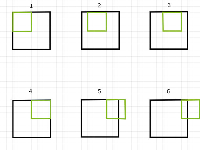
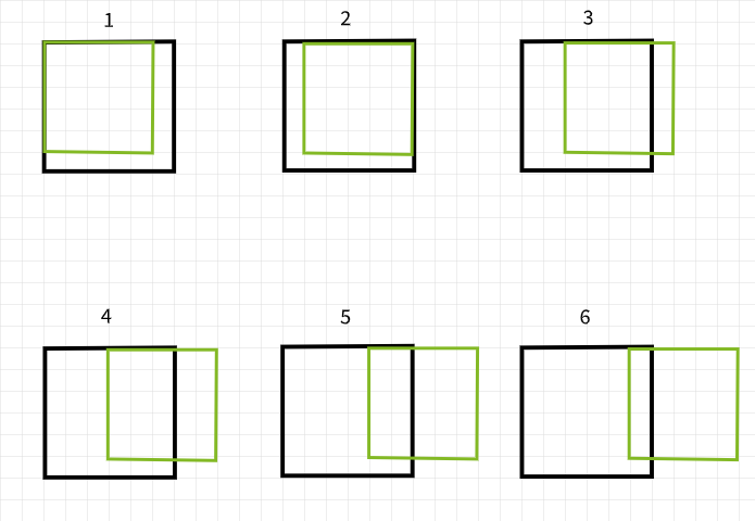
To understand why pixels are lost, bare in mind that if a convolution filter falls out of bounds when scanning over an image, that particular convolution instance is ignored. To illustrate, consider a 6 x 6 pixel image being convolved upon by a 3 x 3 filter. As can be seen in the image below, the first 4 convolutions fall within the image to produce 4 pixels for the first row while the 5th and 6th instances fall out of bounds and are therefore ignored. Likewise, if the filter is shifted downwards by 1 pixel, the same pattern is repeated with a loss of 2 pixels for the second row as well. When the process is complete, the 6 x 6 pixel image becomes a 4 x 4 pixel image since it would have lost 2 columns of pixels in dim 0 (x) and 2 rows of pixels in dim 1 (y).

Likewise, if a 5 x 5 filter is used, 4 columns and rows of pixels are lost in both dim 0 (x) and dim 1 (y) respectively resulting in a 2 x 2 pixel image.

Don't take my word for it, try the function below to see if this is truly the case. Feel free to adjust arguments as desired.

import numpy as np
import torch
import torch.nn.functional as F
import cv2
import torch.nn as nn
from tqdm import tqdm
import matplotlib.pyplot as plt


def check_convolution(filter=(3,3), image_size=(6,6)):
    """
    This function creates a pseudo image, performs
    convolution and returns the size of both the pseudo
    and convolved image
    """
    #  creating pseudo image
    original_image = torch.ones(image_size)
    #  adding channel as typical to images (1 channel = grayscale)
    original_image = original_image.view(1, 6, 6)

    #  perfoming convolution
    conv_image = nn.Conv2d(1, 1, filter)(original_image)

    print(f'original image size: {original_image.shape}')
    print(f'image size after convolution: {conv_image.shape}')
    pass

check_convolution()

There seems to be a pattern to the way pixels are lost. It seems whenever a m x n filter is used, m-1 columns of pixels are lost in dim 0 and n-1 rows of pixels are lost in dim 1. Let's get tad bit more mathematical...

image size = (x, y)
filter size = (m, n)
image size after convolution = (x-(m-1), y-(n-1)) = (x-m+1, y-n+1)

Whenever an image of size (x, y) is convolved using a filter of size (m, n), an image of size (x-m+1, y-n+1) is produced.

While that equation might seem a bit convoluted (no pun intended), the logic behind it is quite simple to follow. Since most common filters are square in size (same dimensions in both axes), all there is to know is that once convolution is done using a (3, 3) filter, 2 rows and columns of pixels are lost (3-1); if it's done using a (5, 5) filter, 4 rows and columns of pixels are lost (5-1); and if it's done using a (9, 9) filter, you guessed it, 8 rows and columns of pixels are lost (9-1).

Implication of Lost Pixels

Losing 2 rows and columns of pixels might not seem to have that much of an effect particularly when dealing with large images, for instance, a 4K UHD image (3840, 2160) would appear unaffected by the loss of 2 rows and columns of pixels when convolved upon by a (3, 3) filter as it becomes (3838, 2158), a loss of about 0.1% of its total pixels. Problems begin to set in when multiple layers of convolution are involved as is typical in state of the art CNN architectures. Take RESNET 128 for instance, this architecture has about 50 (3, 3) convolution layers, that would result in a loss of about 100 rows and columns of pixels, reducing image size to (3740, 2060), a loss of approximately 7.2% of the image's total pixels, all without factoring in downsampling operations.

Even with shallow architectures, losing pixels could have a huge effect. A CNN with just 4 convolution layers applied used on an image in the MNIST dataset with size (28, 28) would result in a loss of 8 rows and columns of pixels, reducing its size to (20, 20), a loss of 57.1% of its total pixels which is quite considerable.

Since convolution operations take place from left to right and top to bottom, pixels are lost at the rightmost and bottom edges. Therefore it's safe to say that convolution results in the loss of edge pixels, pixels which might contain features essential to the computer vision task at hand.

Padding as a Solution

Since we know pixels are bound to be lost after convolution, we can preempt this by adding pixels beforehand. For example, if a (3, 3) filter is going to be used, we could add 2 rows and 2 columns of pixels to the image beforehand so that when convolution is done the image size is the same as the original image.

Let's get a bit mathematical again...

image size = (x, y)
filter size = (m, n)

image size after padding = (x+2, y+2)

using the equation ==> (x-m+1, y-n+1)

image size after convolution (3, 3) = (x+2-3+1, y+2-3+1) = (x, y)

Padding in Layer Terms

Since we are dealing with numeric datatypes, it makes sense for the value of the additional pixels to also be numeric. The common value adopted is a pixel value of zero hence why the term 'zero padding' is often used.

The catch to preemptively adding rows and columns of pixels to an image array is that it has to be done evenly on both sides. For instance, when adding 2 rows and 2 columns of pixels, they should be added as one row at the top, one row at the bottom, one column on the left and one column on the right.

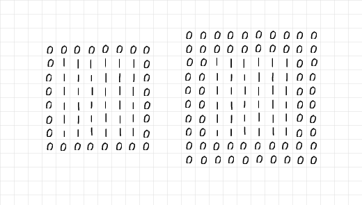
Looking at the image below, 2 rows and 2 columns have been added to pad the 6 x 6 array of ones on the left, while 4 rows and 4 columns have been added on the right. The additional rows and columns have been distributed evenly along all edges as stated in the previous paragraph.

Taking a keen look at the arrays, on the left, it seems like the 6 x 6 array of ones has been enclosed in a single layer of zeros, so padding=1. On the other hand, the array on the right seems to have been enclosed in two layers of zeros, hence padding=2.  

Putting all of these together, it is safe to say that when one is looking to add 2 rows and 2 columns of pixels in preparation for (3, 3) convolution, one needs a single layer of padding. In the same vane, if one needs to add 6 rows and 6 columns of pixels in preparation for (7, 7) convolution, one needs 3 layers of padding. In more technical terms,

Given a filter of size (m, n), (m-1)/2 layers of padding are required to keep image size the same after convolution; provided m=n and m is an odd number.

The Padding Process

To demonstrate the padding process, I have written some vanilla code to replicate the process of padding and convolution.

Firstly, let's take a look at the padding function below, the function takes in an image as parameter with a default padding layer of 2. When the display parameter is left as True, the function generates a mini report by display the size of both the original and padded image; a plot of both images is also returned.

def pad_image(image_path, padding=2, display=True, title=''):
      """
      This function performs zero padding using the number of 
      padding layers supplied as argument and return the padded
      image.
      """
      
      #  reading image as grayscale
      image = cv2.imread(image_path, cv2.IMREAD_GRAYSCALE)
      
      #  creating an array of zeros
      padded = arr = np.zeros((image.shape[0] + padding*2, 
                               image.shape[1] + padding*2))

      #  inserting image into zero array
      padded[int(padding):-int(padding), 
             int(padding):-int(padding)] = image

      if display:
        print(f'original image size: {image.shape}')
        print(f'padded image size: {padded.shape}')

        #  displaying results
        figure, axes = plt.subplots(1,2, sharey=True, dpi=120)
        plt.suptitle(title)
        axes[0].imshow(image, cmap='gray')
        axes[0].set_title('original')
        axes[1].imshow(padded, cmap='gray')
        axes[1].set_title('padded')
        axes[0].axis('off')
        axes[1].axis('off')
        plt.show()
        print('image array preview:')  
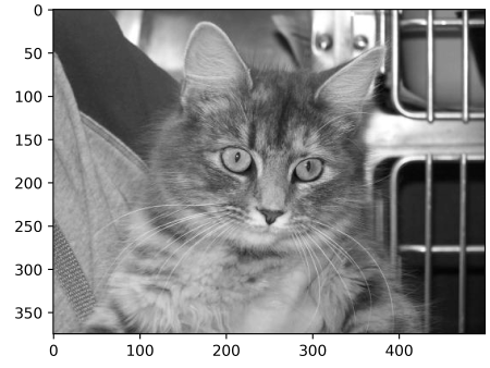
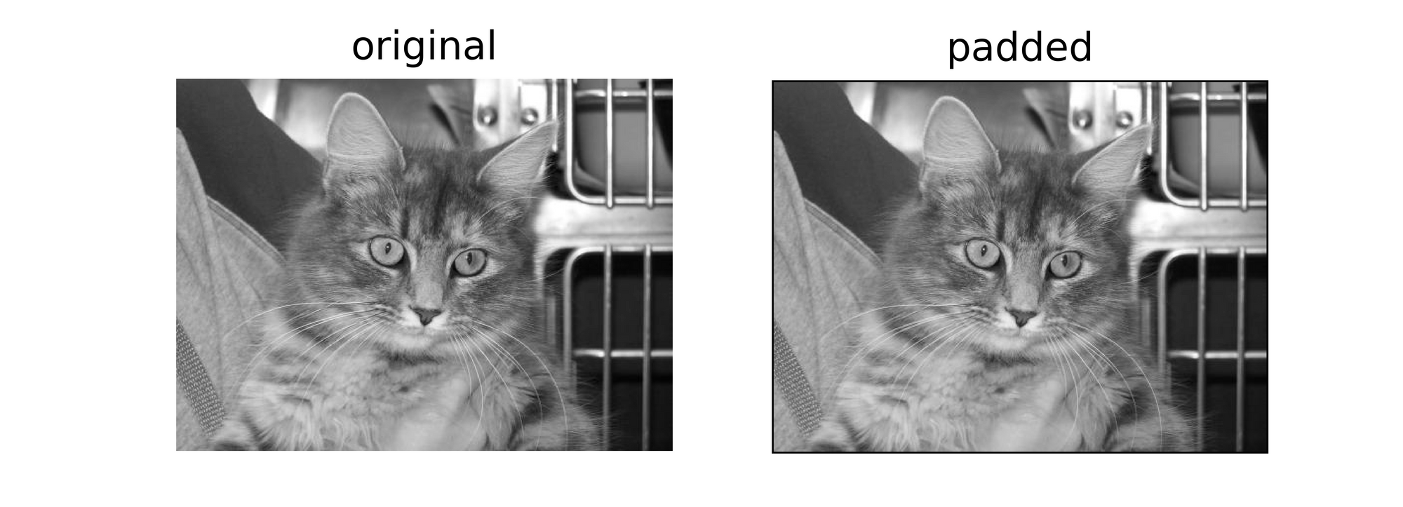
      return padded

To test out the padding function, consider the image below of size (375, 500). Passing this image through the padding function with padding=2 should yield the same image with two columns of zero on the left and right edge and two rows of zeros on the top and bottom increasing the image size to (379, 504). Let's see if this is the case...

pad_image('image.jpg')

output:
original image size: (375, 500)
padded image size: (379, 504)

It works! Feel free to try the function out on any image you might find and adjust parameters as required. Below is vanilla code to replicate convolution.

def convolve(image_path, padding=2, filter, title='', pad=False):
      """
      This function performs convolution over an image 
      """
      
      #  reading image as grayscale
      image = cv2.imread(image_path, cv2.IMREAD_GRAYSCALE)
      
      if pad:
        original_image = image[:]
        image = pad_image(image, padding=padding, display=False)
      else:
        image = image

      #  defining filter size
      filter_size = filter.shape[0]

      #  creating an array to store convolutions
      convolved = np.zeros(((image.shape[0] - filter_size) + 1, 
                        (image.shape[1] - filter_size) + 1))

      #  performing convolution
      for i in tqdm(range(image.shape[0])):
        for j in range(image.shape[1]):
          try:
            convolved[i,j] = (image[i:(i+filter_size), j:(j+filter_size)] * filter).sum()
          except Exception:
            pass

      #  displaying results
      if not pad:
        print(f'original image size: {image.shape}')
      else:
        print(f'original image size: {original_image.shape}')
      print(f'convolved image size: {convolved.shape}')

      figure, axes = plt.subplots(1,2, dpi=120)
      plt.suptitle(title)
      if not pad:
        axes[0].imshow(image, cmap='gray')
        axes[0].axis('off')
      else:
        axes[0].imshow(original_image, cmap='gray')
        axes[0].axis('off')
      axes[0].set_title('original')
      axes[1].imshow(convolved, cmap='gray')
      axes[1].axis('off')
      axes[1].set_title('convolved')
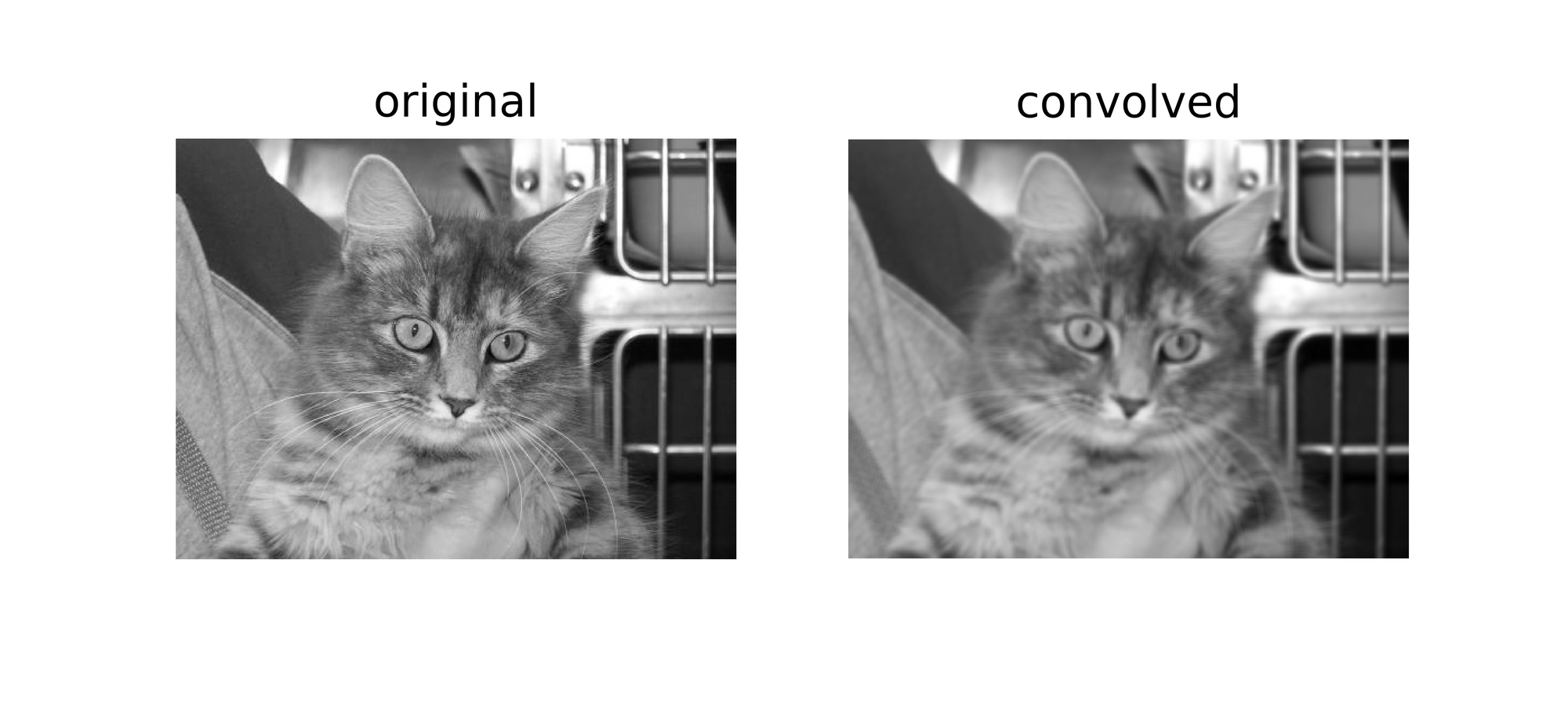
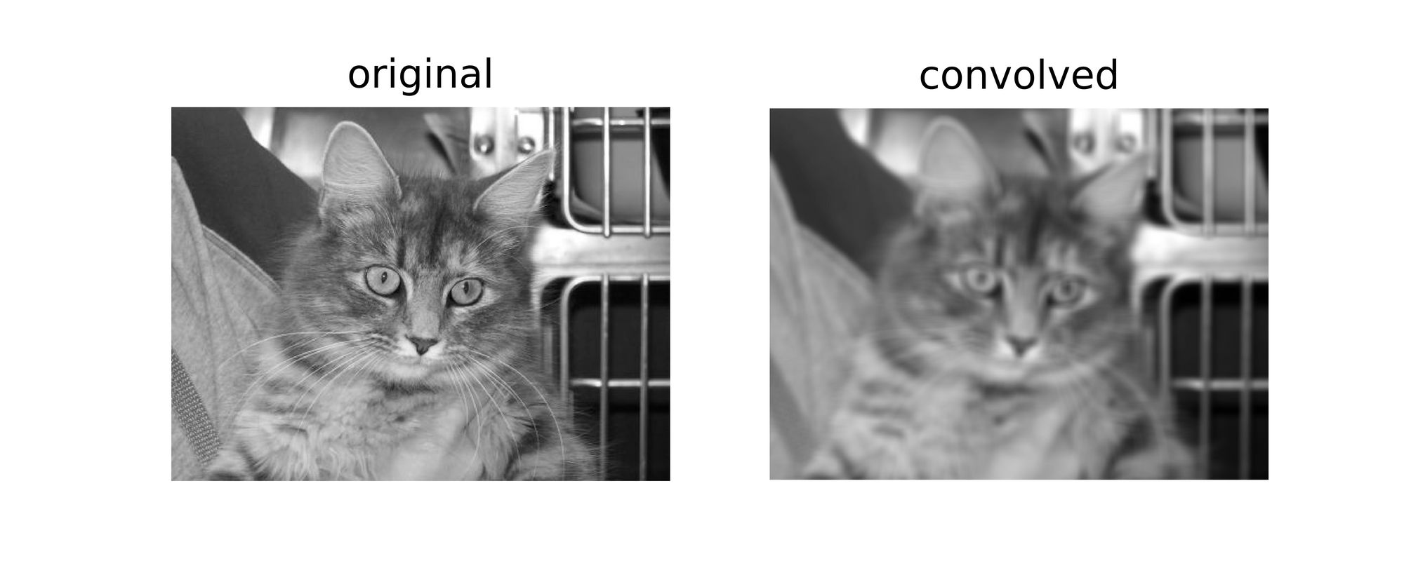
      pass

For the filter I've chosen to go with a (5, 5) array with values of 0.01. The idea behind this is for the filter to reduce pixel intensities by 99% before summing to produce a single pixel. In simplistic terms, this filter should have a blurring effect on images.

filter_1 = np.ones((5,5))/100

filter_1
[[0.01, 0.01, 0.01, 0.01, 0.01]
 [0.01, 0.01, 0.01, 0.01, 0.01]
 [0.01, 0.01, 0.01, 0.01, 0.01]
 [0.01, 0.01, 0.01, 0.01, 0.01]
 [0.01, 0.01, 0.01, 0.01, 0.01]]

Applying the filter on the original image without padding should yield a blurred image of size (371, 496), a loss of 4 rows and 4 columns.

convolve('image.jpg', filter=filter_1)

output:
original image size: (375, 500)
convolved image size: (371, 496)

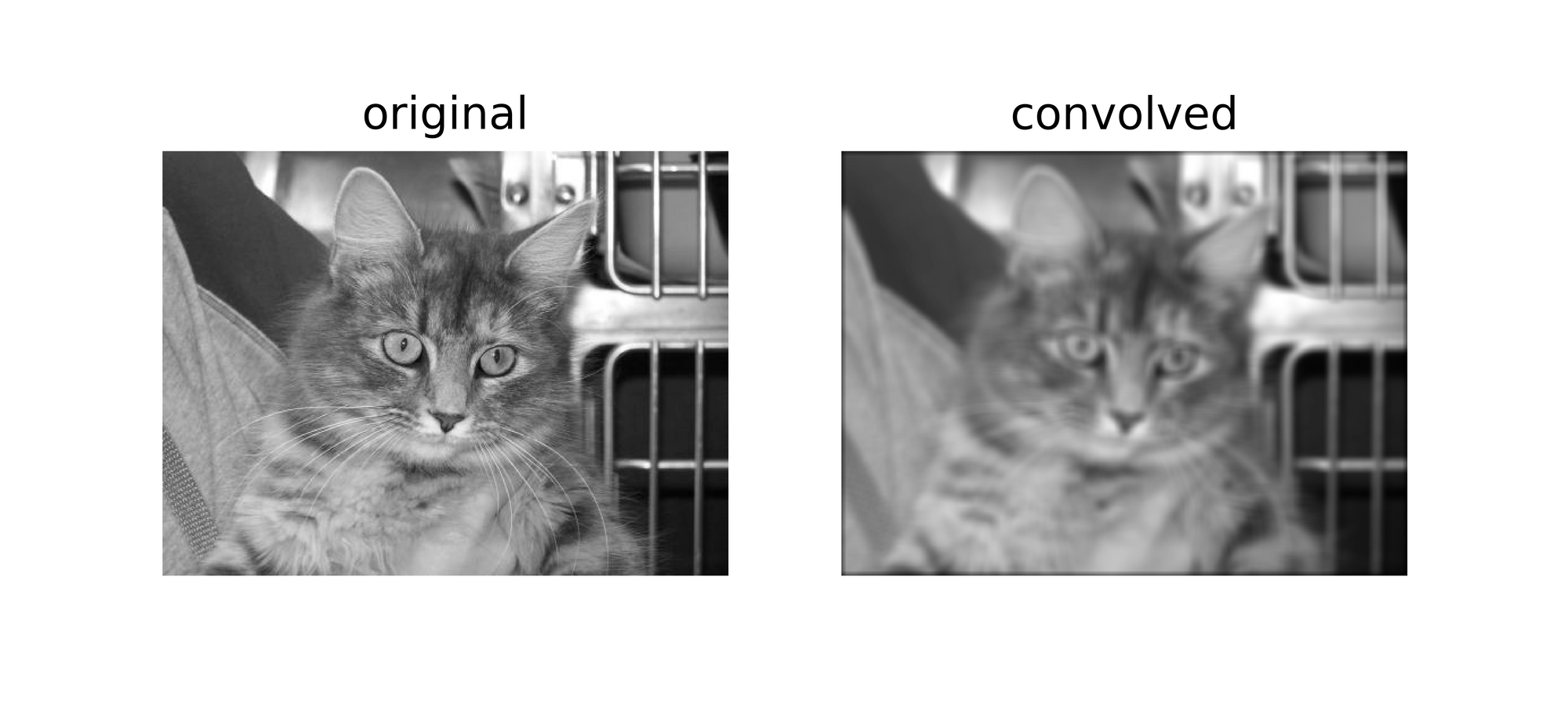
However when pad is set to true, the image size remains the same.

convolve('image.jpg', pad=True, padding=2, filter=filter_1)

output:
original image size: (375, 500)
convolved image size: (375, 500)

Let's repeat the same steps but with a (9, 9) filter this time...

filter_2 = np.ones((9,9))/100
filter_2

filter_2
[[0.01, 0.01, 0.01, 0.01, 0.01, 0.01, 0.01, 0.01, 0.01],
 [0.01, 0.01, 0.01, 0.01, 0.01, 0.01, 0.01, 0.01, 0.01],
 [0.01, 0.01, 0.01, 0.01, 0.01, 0.01, 0.01, 0.01, 0.01],
 [0.01, 0.01, 0.01, 0.01, 0.01, 0.01, 0.01, 0.01, 0.01],
 [0.01, 0.01, 0.01, 0.01, 0.01, 0.01, 0.01, 0.01, 0.01],
 [0.01, 0.01, 0.01, 0.01, 0.01, 0.01, 0.01, 0.01, 0.01],
 [0.01, 0.01, 0.01, 0.01, 0.01, 0.01, 0.01, 0.01, 0.01],
 [0.01, 0.01, 0.01, 0.01, 0.01, 0.01, 0.01, 0.01, 0.01],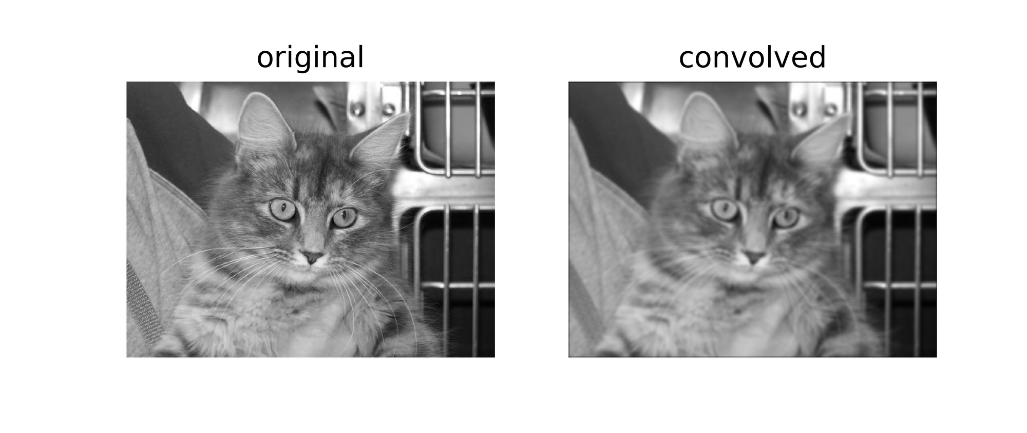
 [0.01, 0.01, 0.01, 0.01, 0.01, 0.01, 0.01, 0.01, 0.01]])

Without padding the resulting image reduces in size...

convolve('image.jpg', filter=filter_2)

output:
original image size: (375, 500)
convolved image size: (367, 492)

Using a (9, 9) filter, in order to keep image size the same we need to specify a padding layer of 4 (9-1/2) since we will be looking to add 8 rows and 8 columns to the original image.

convolve('image.jpg', pad=True, padding=4, filter=filter_2)

output:
original image size: (375, 500)
convolved image size: (375, 500)

From a PyTorch Perspective

For ease of illustration I had chosen to explain the processes using vanilla code in the section above. The same process can be replicated in PyTorch, bare in mind however that the resulting image will most likely experience little to no transformation as PyTorch will randomly initialize a filter which is not designed for any specific purpose.

To demonstrate this, let's modify the check_convolution() function defined in one of the preceeding sections above...

def check_convolution(image_path, filter=(3,3), padding=0):
    """
    This function performs convolution on an image and 
    returns the size of both the original and convolved image
    """
    
    image = cv2.imread(image_path, cv2.IMREAD_GRAYSCALE)
    
    image = torch.from_numpy(image).float()

    #  adding channel as typical to images (1 channel = grayscale)
    image = image.view(1, image.shape[0], image.shape[1])

    #  perfoming convolution
    with torch.no_grad():
      conv_image = nn.Conv2d(1, 1, filter, padding=padding)(image)

    print(f'original image size: {image.shape}')
    print(f'image size after convolution: {conv_image.shape}')
    pass

Notice that in the function I used the default PyTorch 2D convolution class and the function's padding parameter is directly supplied to the convolution class. Now let's try different filters and see what the resulting image sizes are...

check_convolution('image.jpg', filter=(3, 3))

output:
original image size: torch.Size(1, 375, 500)
image size after convolution: torch.Size(1, 373, 498)

check_convolution('image.jpg', filter=(3, 3), padding=1)

output:
original image size: torch.Size(1, 375, 500)
image size after convolution: torch.Size(1, 375, 500)

check_convolution('image.jpg', filter=(5, 5))

output:
original image size: torch.Size(1, 375, 500)
image size after convolution: torch.Size(1, 371, 496)

check_convolution('image.jpg', filter=(5, 5), padding=2)

output:
original image size: torch.Size(1, 375, 500)
image size after convolution: torch.Size(1, 375, 500)

As evident in the examples above, when convolution is done without padding, the resulting image is of a reduced size. However, when convolution is done with the correct amount of padding layers, the resulting image is equal in size to the original image.

Final Remarks

In this article we have been able to ascertain that the convolution process does in fact result in a loss of pixels. We have also been able to prove that preemptively adding pixels to an image, in a process calling padding, before convolution ensures that the image retains its original size after convolution.