Winning Hearts: Love Island’s Love Algorithm

When it comes to learning from data, we often default to learning from tabular data. And yet, data assumes many structures. The graph data structure is one that’s frequently overlooked. Why is this?

Most are familiar with data tables. As the incumbent data structure, tabular data enjoys an extensive ecosystem of tools and technologies. So that’s all there is to it? It’s the established norm? I think we can do better.

Recently, the field has witnessed significant advancements to graph learning, sparking interest within the machine learning community. The community seems to recognize the transformative potential of training on data representations that encapsulate the depth and complexity of relationships. Leveraging graph learning fosters insights and facilitates innovative solutions across diverse domains.

Graph Data Structures

Graph data is information modeled using a graph data structure. A graph data structure consists of two fundamental components: nodes and edges.

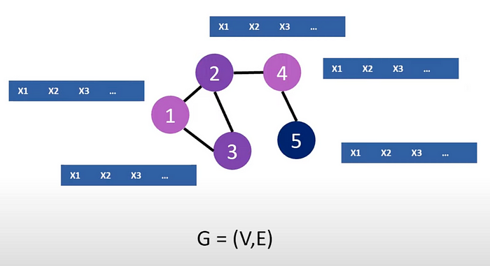
• Each node, or vertex (V), represents a data entity.
  ​ ​ ​​​ ​​ ​​​ ​ — A node would be equivalent to a row of tabular data.
• Each edge (E) represents a connection between nodes.

In graph theory, G = (V, E) is common notation used to represent a graph (G).

The Show

Putting theoretical concepts to practice, in this tutorial we’ll train a Graph Convolutional Network using data from our favorite reality TV show, Love Island.

Picture this: a lavish villa, a tropical island and a group of sun-kissed singles. In their quest for love, islanders “couple up”, and together, take on challenges designed to test their romantic connections. But here’s the twist — you’re not just a spectator. You have the power to shape these islanders’ destinies by voting for your favorite couples.

With a deeper understanding of the show’s dynamics, we begin to see that it’s not only the connections formed amongst the islanders that matter. Public opinion plays a significant role in determining their fate on the show. Equipped with this domain knowledge, we can now better approach problem formulation and data collection.

The Data

Data collection is a critical phase of every data project, and frequently constitutes the majority of the workload. For this project, we’ll work with two datasets; one encompassing data on public sentiment and the other containing information on islander couples.

Public Sentiment

Without access to the public vote for their favorite couples, we’ll assess public sentiment for each islander using a dataset of tweets. The number of mentions for each islander will serve to measure public sentiment–a resourceful solution to the data constraints seen with this, and with so many other, data projects.

Couples

In addition to our dataset on public sentiment, we’ll also need data on the relationships formed between the islanders, specifically, on the couples.

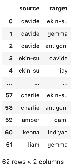
Leveraging this connection information, the subsequent code will construct a network using the networkx library. We display that network below.

import networkx as nxG = nx.Graph()for idx, row in connections_df.iterrows():
    source = row['source']
    target = row['target']
    G.add_edge(source, target)nx.draw(G, with_labels = True)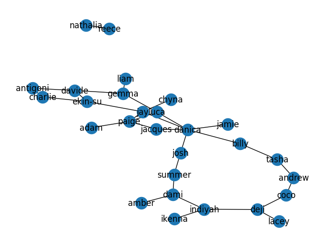

Graph Convolutional Networks

Now let’s shift our focus to the frameworks designed to learn from graph data. There are many, and Graph Convolutional Networks (GCNs) have emerged as the most prevalent technology. Graph Convolutional Networks (GCNs) consist of successive layers, known as message passing layers.

Message passing layers, integral to GCNs, are fundamental components responsible for consolidating node and edge data to the model’s node embeddings. Node embeddings, which represent nodes in the graph, are obtained through information aggregation from neighboring nodes, the node’s own features, and possibly edge features.

GCNs facilitate tasks like node classification, where the objective is to assign labels to graph nodes. In the code that follows, we train a GCN to classify our islanders, represented as nodes, as winners (1) or runner-ups (0).

Copy and paste this in a code cell using the Run on Paperspace link above:

import torch
from torch_geometric.utils.convert import to_networkx, from_networkx
import torch_geometric.transforms as T
from torch_geometric.nn import GCNConv
import torch.nn.functional as F

# Check if a GPU (cuda) is available; if not, use the CPU
device = torch.device('cuda' if torch.cuda.is_available() else 'cpu')

# Convert the graph into PyTorch Geometric Data object
graph = from_networkx(G)
# Create RandomNodeSplit Object to split graph to train, test and validation datasets
split = T.RandomNodeSplit(num_val=0.1, num_test=0.2)
data = split(graph)

# Reshape feature vector to have dimensions (28, 1)
data.x = data.x.view(28, 1)
# Convert 'data.y' to type LongTensor, typically used for classification targets
data.y = data.y.type(torch.LongTensor)

# Get the shape of the feature vector
feature_shape = data.x.shape # torch.Size([28, 1])
num_features = feature_shape[1]
# Find unique target values and their counts for the target vector
target_shape = data.y.unique(return_counts=True) # (tensor([0, 1]), tensor([20,  8]))
num_classes = len(target_shape[1])

# Define a Graph Convolutional Network (GCN) model
class GCN(torch.nn.Module):
    def __init__(self, hidden_channels):
        super().__init__()
        torch.manual_seed(1)
        # Create the first graph convolutional layer with 'num_features' input channels and 'hidden_channels' output channels
        self.conv1 = GCNConv(num_features, hidden_channels)
        # Create the second graph convolutional layer with 'hidden_channels' input channels and 'num_classes' output channels
        self.conv2 = GCNConv(hidden_channels, num_classes)    def forward(self, x, edge_index):
        x = self.conv1(x, edge_index)
        x = x.relu()
        # Apply dropout with a probability of 0.5 (used during training)
        x = F.dropout(x, p=0.5, training=self.training)
        # Apply the second graph convolutional layer
        x = self.conv2(x, edge_index)
        return x
        
# Create an instance of the GCN model with 'hidden_channels' set to 16
model = GCN(hidden_channels=16)

# Define the optimizer for training the model (Adam optimizer)
optimizer = torch.optim.Adam(model.parameters(), lr=0.01, weight_decay=5e-4)
# Define the loss criterion (CrossEntropyLoss) for training
criterion = torch.nn.CrossEntropyLoss()

def train():
  # Train the model
  model.train()
  # Zero out the gradients
  optimizer.zero_grad()
  out = model(data.x, data.edge_index)
  # Calculate the loss using the specified criterion
  loss = criterion(out[data.train_mask], data.y[data.train_mask])
  # Backpropagate the gradients
  loss.backward()
  # Update model weights using the optimizer
  optimizer.step()
  # Return the computed loss for this training step
  return loss

def test():
  model.eval()
  out = model(data.x, data.edge_index)
  # Determine the predicted class by the highest probability
  pred = out.argmax(dim=1)
  # Compare the predicted classes with the true classes for test-masked elements
  test_correct = pred[data.test_mask] == data.y[data.test_mask]
  # Calculate the test accuracy as the ratio of correct predictions to total test-masked elements
  test_acc = int(test_correct.sum()) / int(data.test_mask.sum())
  return test_acc
  
for epoch in range(1, 10):
  loss = train()
  
test_acc = test()
print(f'Test Accuracy: {test_acc:.4f}')

Because our network is small, our validation set consists of just 3 nodes. Across numerous trials, our model consistently achieves a 67% accuracy rate, i.e. correctly predicts 2 of the 3 nodes.

This has been a simple demonstration of graph learning. We represented islanders and their characteristics as nodes and node features, and trained a GCN to learn from the connections formed amongst the islanders to predict the reality tv show winners.

There’s a wealth of untapped potential in graph learning. Stay tuned for more fascinating applications!