Bring this project to life
Object detection is undoubtedly one of the "Holy Grails" of deep learning technology's promise. The practice of combining image classification and object identification, object detection involves identifying the location of a discrete object in an image and correctly classifying it. Bounding boxes are then predicted and placed within a copy of the image, so that the user can directly see the model's predicted classifications.
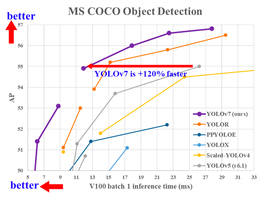
YOLO has remained one of the premiere object detection networks since its creation for two primary reasons: it's accuracy, relatively low cost, and ease of use. These traits together have made YOLO undoubtedly one of the most famous DL models outside of the data science community at large due to this utile combination. Having undergone multiple iterations of development, YOLOv7 is the latest version of the popular algorithm, and improves significantly on its predecessors.
In this blog tutorial, we will start by examining the greater theory behind YOLO's action, its architecture, and comparing YOLOv7 to its previous versions. We will then jump into a coding demo detailing all the steps you need to develop a custom YOLO model for your object detection task. We will use NBA game footage as our demo dataset, and attempt to create a model that can distinguish and label the ball handler separately from the rest of the players on the court.
What is YOLO?
The original YOLO model was introduced in the paper “You Only Look Once: Unified, Real-Time Object Detection” in 2015. At the time, RCNN models were the best way to perform object detection, and their time consuming, multi-step training process made them cumbersome to use in practice. YOLO was created to do away with as much of that hassle as possible, by offering single-stage object detection they reduced training & inference times as well as massively reduced the cost to run object detection.
Since then, various groups have tackled YOLO with the intention of making improvements. Some examples of these new versions include the powerful YOLOv5 and YOLOR. Each of these iterations attempted to improve upon past incarnations, and YOLOv7 is now the highest performant model of the family with its release.
How does YOLO work?
YOLO works to perform object detection in a single stage by first separating the image into N grids. Each of these grids is of equal size SxS. Each of these regions is used to detect and localize any objects they may contain. For each grid, bounding box coordinates, B, for the potential object(s) are predicted with an object label and a probability score for the predicted object's presence.
As you may have guessed, this leads to a significant overlap of predicted objects from the cumulative predictions of the grids. To handle this redundancy and reduce the predicted objects down to those of interest, YOLO uses Non-Maximal Suppression to suppress all the bounding boxes with comparatively lower probability scores.

To achieve this, YOLO first compares the probability scores associated with each decision, and takes the largest score. Following this, it removes the bounding boxes with the largest Intersection over Union with the chosen high probability bounding box. This step is then repeated until only the desired final bounding boxes remain.
What changes were made in YOLOv7
A number of new changes were made for YOLOv7. This section will attempt to breakdown these changes, and show how these improvements lead to the massive boost in performance in YOLOv7 compared to predecessor models.
Extended efficient layer aggregation networks
Model re-paramaterization is the practice of merging multiple computational models at the inference stage in order to accelerate inference time. In YOLOv7, the technique "Extended efficient layer aggregation networks" or E-ELAN is used to perform this feat.
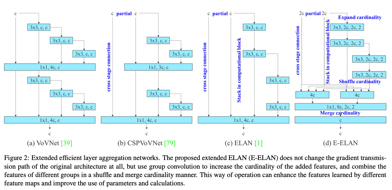
E-ELAN implements expand, shuffle, and merge cardinality techniques to continuously improve the adaptability and capability to learn of the network without having an effect on the original gradient path. The goal of this method is to use group convolution to expand the channel and cardinality of computational blocks. It does so by applying the same group parameter and channel multiplier to each computational block in the layer. The feature map is then calculated by the block, and shuffled into a number of groups, as set by the variable g, and combined. This way, the amount of channels in each group of feature maps is the same as the number of channels in the original architecture. We then add the groups together to merge cardinality. By only changing the model architecture in the computational block, the transition layer is left unaffected and the gradient path is fixed. [Source]
Model scaling for concatenation-based models
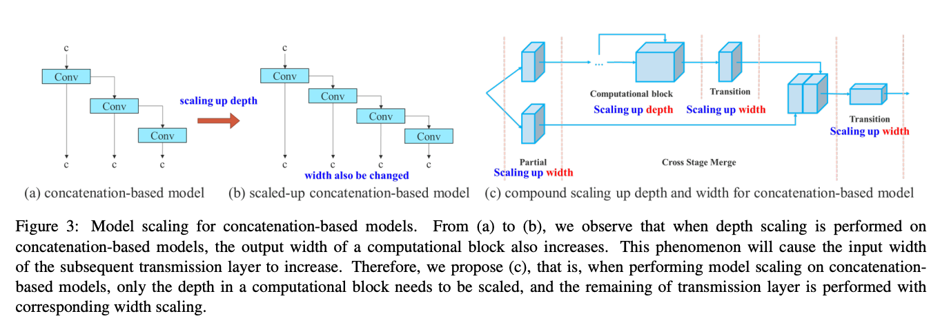
It is common for YOLO and other object detection models to release a series of models that scale up and down in size, to be used in different use cases. For scaling, object detection models need to know the depth of the network, the width of the network, and the resolution that the network is trained on. In YOLOv7, the model scales the network depth and width simultaneously while concatenating layers together. Ablation studies show that this technique keeps the model architecture optimal while scaling for different sizes. Normally, something like scaling-up depth will cause a ratio change between the input channel and output channel of a transition layer, which may lead to a decrease in the hardware usage of the model. The compound scaling technique used in YOLOv7 mitigates this and other negative effects on performance made when scaling.
Trainable bag of freebies
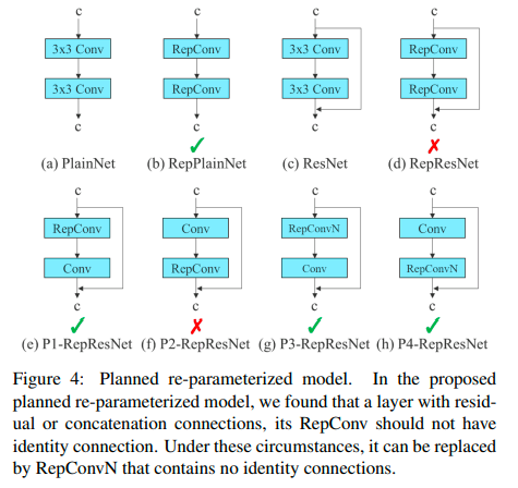
The YOLOv7 authors used gradient flow propagation paths to analyze how re-parameterized convolution should be combined with different networks. The above diagram shows in what way the convolutional blocks should be placed, with the check marked options representing that they worked.
Coarse for the auxiliary heads, and fine for the lead loss head
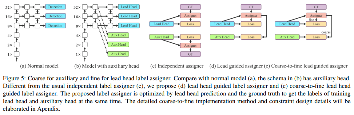
Deep supervision a technique that adds an extra auxiliary head in the middle layers of the network, and uses the shallow network weights with assistant loss as the guide. This technique is useful for making improvements even in situations where model weights typically converge. In the YOLOv7 architecture, the head responsible for the final output is called the lead head, and the head used to assist in training is called the auxiliary head. YOLOv7 uses the lead head prediction as guidance to generate coarse-to-fine hierarchical labels, which are used for auxiliary head and lead head learning, respectively.
All together, these improvements have lead to the significant increases in capability and decreases in cost we saw in the above diagram when compared to its predecessors.
Setting up your custom datasets
Now that we understand why and how YOLOv7 is such an improvement over past techniques, we can try it out! For this demo, we are going to download videos of NBA highlights, and create a YOLO model that can accurately detect which players on the court are actively holding the ball. The challenge here is to get the model to capably and reliably detect and discern the ball handler from the other players on the court. To do this, we can go to Youtube and download some NBA highlight reels. We can then use VLC's snapshot filter to breakdown the videos into sequences of images.
To continue on to training, you will first need to choose an appropriate labeling tool to label the newly made custom dataset. YOLO and related models require that the data used for training has each of the desired classifications accurately labeled, usually by hand. We chose to use RoboFlow for this task. The tool is free to use online, quick, can perform augmentations and transformations on uploaded data to diversify the dataset, and can even freely triple the amount of training data based on the input augmentations. The paid version comes with even more useful features.
Create a RoboFlow account, start a new project, and then upload the relevant data to the project space.
The two possible classifications that we will use for this task are 'ball-handler' and 'player.' To label the data with RoboFlow once it is uploaded, all you need to do is click the "Annotate" button on the left hand menu, click on the dataset, and then drag your bounding boxes over the desired objects, in this case basketball players with and without the ball.
This data is composed entirely of in game footage, and all commercial break or heavily 3d CGI filled frames were excluded from the final dataset. Each player on the court was identified as 'player', the label for the majority of the bounding box classifications in the dataset. Nearly every frame, but not all, also included a 'ball-handler'. The 'ball-handler' is the player currently in possession of the basketball. To avoid confusion, the ball handler is not double labeled as a player in any frames. To attempt to account for different angles used in game footage, we included angles from all shots and maintained the same labeling strategy for each angle. Originally, we attempted a separate 'ball-handler-floor' and 'player-floor' tag when footage was shot from the ground, but this only added confusion to the model.
Generally speaking, it is suggested that you have 2000 images for each type of classification. It is, however, extremely time consuming to label so many images, each with many objects, by hand, so we are going to use a smaller sample for this demo. It still works reasonably well, but if you wish to improve on this models capability, the most important step would be to expose it to more training data and a more robust validation set.
We used 1668 (556x3) training photos for our training set, 81 images for the test set, and 273 images for the validation set. In addition to the test set, we will create our own qualitative test to assess the model's viability by testing the model on a new highlight reel. You can generate your dataset using the generate button in RoboFlow, and then get it output to your Notebook through the curl terminal command in the YOLOv7 - PyTorch format. Below is the code snippet you could use to access the data used for this demo:
curl -L "https://app.roboflow.com/ds/4E12DR2cRc?key=LxK5FENSbU" > roboflow.zip; unzip roboflow.zip; rm roboflow.zip
Code demo
You can run all the code needed for this demo by clicking the link below.
Bring this project to life
Setup
To get started with the code demo, simply click the run on gradient link below. Once your Notebook has finished set up and is running, navigate to 'notebook.ipynb.' This notebook contains all the code needed to set up your model. The file 'data/coco.yaml' is configured to work with our data.
First, we will load in the required data and the model baseline we will fine-tune:
!curl -L "https://app.roboflow.com/ds/4E12DR2cRc?key=LxK5FENSbU" > roboflow.zip; unzip roboflow.zip; rm roboflow.zip
!wget https://github.com/WongKinYiu/yolov7/releases/download/v0.1/yolov7_training.pt
! mkdir v-test
! mv train/ v-test/
! mv valid/ v-test/
Next, we have a few required packages that need to be installed, so running this cell will get your environment ready for training. We are downgrading Torch and Torchvision because YOLOv7 cannot work on the current versions.
!pip install -r requirements.txt
!pip install setuptools==59.5.0
!pip install torchvision==0.11.3+cu111 -f https://download.pytorch.org/whl/cu111/torch_stable.html
Helpers
import os

# remove roboflow extra junk

count = 0
for i in sorted(os.listdir('v-test/train/labels')):
    if count >=3:
        count = 0
    count += 1
    if i[0] == '.':
        continue
    j = i.split('_')
    dict1 = {1:'a', 2:'b', 3:'c'}
    source = 'v-test/train/labels/'+i
    dest = 'v-test/train/labels/'+j[0]+dict1[count]+'.txt'
    os.rename(source, dest)

count = 0
for i in sorted(os.listdir('v-test/train/images')):
    if count >=3:
        count = 0
    count += 1
    if i[0] == '.':
        continue
    j = i.split('_')
    dict1 = {1:'a', 2:'b', 3:'c'}
    source = 'v-test/train/images/'+i
    dest = 'v-test/train/images/'+j[0]+dict1[count]+'.jpg'
    os.rename(source, dest)

for i in sorted(os.listdir('v-test/valid/labels')):
    if i[0] == '.':
        continue
    j = i.split('_')
    source = 'v-test/valid/labels/'+i
    dest = 'v-test/valid/labels/'+j[0]+'.txt'
    os.rename(source, dest)

for i in sorted(os.listdir('v-test/valid/images')):
    if i[0] == '.':
        continue
    j = i.split('_')
    source = 'v-test/valid/images/'+i
    dest = 'v-test/valid/images/'+j[0]+'.jpg'
    os.rename(source, dest)
for i in sorted(os.listdir('v-test/test/labels')):
    if i[0] == '.':
        continue
    j = i.split('_')
    source = 'v-test/test/labels/'+i
    dest = 'v-test/test/labels/'+j[0]+'.txt'
    os.rename(source, dest)

for i in sorted(os.listdir('v-test/test/images')):
    if i[0] == '.':
        continue
    j = i.split('_')
    source = 'v-test/test/images/'+i
    dest = 'v-test/test/images/'+j[0]+'.jpg'
    os.rename(source, dest)
The next section of the notebook aids in setup. Because RoboFlow data outputs with an additional string of data and id's appended to the end of the filename, we first remove all of the extra text. These would have prevented training from running as they differ from jpg to corresponding txt file. The training files are also in triplicate, which is why the training rename loop contains additional steps.
Train
Now that our data is setup, we are ready to start training our model on our custom dataset. We used a 2 x A6000 model to train our model for 50 epochs. The code for this part is simple:
# Train on single GPU
!python train.py --workers 8 --device 0 --batch-size 8 --data data/coco.yaml --img 1280 720 --cfg cfg/training/yolov7.yaml --weights yolov7_training.pt --name yolov7-ballhandler --hyp data/hyp.scratch.custom.yaml --epochs 50

# Train on 2 GPUs
!python -m torch.distributed.launch --nproc_per_node 2 --master_port 9527 train.py --workers 16 --device 0,1 --sync-bn --batch-size 8 --data data/coco.yaml --img 1280 720 --cfg cfg/training/yolov7.yaml --weights yolov7_training.pt --name yolov7-ballhandler --hyp data/hyp.scratch.custom.yaml --epochs 50
We have provided two methods for running training on a single GPU or multi-GPU system. By executing this cell, training will begin using the desired hardware. You can modify these parameters here, and, additionally, you can modify the hyperparameters for YOLOv7 at 'data/hyp.scratchcustom.yaml'. Let's go over some of the more important of these parameters.
- workers (int): how many subprocesses to parallelize during training
- img (int): the resolution of our images. For this project, the images were resized to 1280 x 720
- batch_size (int): determines the number of samples processed before the model update is created
- nproc_per_node (int): number of machines to use during training. For multi-GPU training, this usually refers to the number of available machines to point to.
During training, the model will output the memory reserved for training, the number of images examined, total number of predicted labels, precision, recall, and mAP @.5 at the end of each epoch. You can use this information to help identify when the model is ready to complete training and understand the efficacy of the model on the validation set.
At the end of training, the best, last, and some additional model stages will be saved to the corresponding directory in "runs/train/yolov7-ballhandler[n]", where n is the number of times training has been run. It will also save some relevant data about the training process. You can change the name of the save directory in the command with the --name flag.
Detect
Once model training has completed, we are no able to use the model to perform object detection in realtime. This is able to work on both image and video data, and will output the predictions for you in real time (outside Gradient Notebooks) in the form of the frame including the bounding box(es). We will use detect as our means of qualitatively assessing the efficacy of the model at its task. For this purpose, we downloaded unrelated NBA game footage from Youtube, and uploaded it to the Notebook to use as a novel test set. You can also directly plug in a URL with an HTTPS, RTPS, or RTMP video stream as a URL string, but YOLOv7 may prompt a few additional installs before it can proceed.
Once we have entered our parameters for training, we can call on the detect.py script to detect any of the desired objects in our new test video.
!python detect.py --weights runs/train/yolov7-ballhandler/weights/best.pt --conf 0.25 --img-size 1280 --source video.mp4 --name test
After training for fifty epochs, using the exact same methods described above, you can expect your model to perform approximately like the one shown in the videos below:
Due to the diversity of training image angles used, this model is able to account for all kinds of shots, including floor level and a more distant ground level from the opposite baseline. The vast majority of the shots, the model is able to correctly identify the ball handler, and simultaneously label each additional player on the court.
The model is not perfect, however. We can see that sometimes occlusion of part of a players body while turned around seems to confound the model, as it tries to assign ball handler labels to players in these positions. Often, this occurs while a player's back is turned to the camera, likely due to the frequency this happens for guards setting up plays or while driving to the basket.
Other times, the model identifies multiple players on the court as being in possession, such as during the fast break shown above. It's also notable that dunking and blocking on the close camera view can confuse the model as well. Finally, if a small area of the court is occupied by most of the players, it can obscure the ball handler from the model and cause confusion.
Overall, the model appears to be generally succeeding at detecting each player and ball handler from the perspective of our qualitative view, but suffers from some difficulties in the rarer angles used during certain plays, when the half court is extremely crowded with players, and while doing more athletic plays that aren't accounted for in the training data, like unique dunks. From this, we can surmise that the problem is not the quality of our data nor the amount of training time, but instead the volume of training data. Ensuring a robust model would likely require around 3 times the amount of images as are in the current training set.
Let's now use YOLOv7's built in test program to assess our data on the test set.
Test
The test.py script is the simplest and quickest way to assess the quality of your model using your test set. It rapidly assesses the quality of the predictions made on the test set, and returns them in a legible format. When used in tandem with our qualitative analyses, we gain a fuller understanding of how our model is performing.
RoboFlow suggests a 70-20-10 train-test-validation split of a dataset when used for YOLO, in addition to 2000 images per classification. Since our test set is small, its likely that several classes are underrepresented, so take these results with a grain of salt and use a more robust test set than we chose to for your own projects. Here we use test.yaml instead of coco.yaml.
!python test.py --data data/test.yaml --img 1280 --batch 16 --conf 0.001 --iou 0.65 --device 0 --weights runs/train/yolov7-ballhandler/weights/best.pt --name yolov7_ballhandler_testing
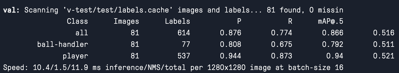
You will then get an output in the log, as well as several figures and data points assessing the efficacy of the model on the test set saved to the prescribed location. In the logs, you can see the total number of images in the folder and the number of labels for each category in those images, and then the precision, recall, and mAP@.5 for both the cumulative predictions and for each type of classification.
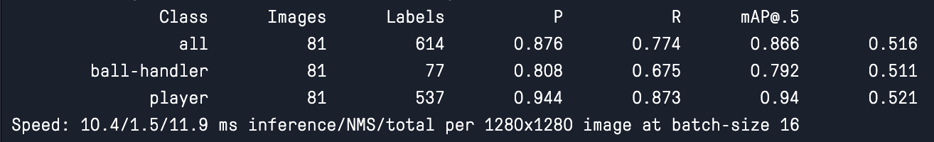
As we can see, the data reflects a healthy model that achieves at least ~ .79 mAP@.5 efficacy at predicting each of the real labels in the test set.
The ball-handler's comparatively lower recall, precision, and mAP@.5, given our distinct class imbalance & the extreme similarity between classes, makes complete sense in the context of how much data was used for training. It is sufficient to say that the quantitative results corroborate our qualitative findings, and that the model is capable but requires more data to reach full utility.
Closing thoughts
As we can see, YOLOv7 is not only a powerful tool for the obvious reasons of accuracy in use, but is also extremely easy to implement with the help of a robust labeling tool like RoboFlow and a powerful GPU like those available on Paperspace Gradient. We chose this challenge because of the apparent difficulty in discerning basketball players with and without the ball for humans, let alone machines. These results are very promising, and already a number of applications for tracking the players for stat keeping, gambling, and player training could easily be derived from this technology.
We encourage you to follow the workflow described in this article on your own custom dataset after running through our prepared version. Additionally, there are a plethora of public and community datasets available on RoboFlow's dataset storage. Be sure to peruse these datasets before beginning the data labeling. Thank you for reading!