Advanced Recurrent Neural Networks: Deep RNNs

This series gives an advanced guide to different recurrent neural networks (RNNs). You will gain an understanding of the networks themselves, their architectures, applications, and how to bring the models to life using Keras.

In this tutorial we’ll start by looking at deep RNNs. Specifically, we’ll cover:

1. The Idea: Speech Recognition
2. Why an RNN?
3. Introducing Depth Into the Network: Deep RNNs
4. The Mathematical Notion
5. Generating Music Using a Deep RNN
6. Conclusion

Let’s get started!

The Idea: Speech Recognition

Speech Recognition is the identification of the text in speech by computers. Speech, as we perceive it, is sequential in nature. If you are to model a speech recognition problem in deep learning, which model do you think suits the task best?

As we'll see, it could very well be a recurrent neural network, or RNN.

Why an RNN?

Handwriting recognition is similar to speech recognition, concerning the data type at least–they both are sequential. Interestingly, RNNs have generated state-of-the-art results in recognizing handwriting as can be seen in Online Handwriting Recognition and Offline Handwriting Recognition research. RNNs have proved to generate efficient outputs with sequential data.

Thus, we might optimistically say that an RNN can best fit a speech recognition model as well.

Yet, unanticipatedly, when a speech recognition RNN model was fit onto the data, the results were not as promising. Deep feedforward neural networks generated better accuracy in comparison to a typical RNN. Although RNNs fared pretty well in handwriting recognition, it wasn’t considered to be a suitable choice for the speech recognition task.

After analyzing why the RNNs failed, researchers proposed a possible solution to attain greater accuracy: by introducing depth into the network, similar to how a deep feed-forward neural network is composed.

Introducing Depth into the Network: Deep RNNs

An RNN is deep with respect to time. But what if it’s deep with respect to space as well, as in a feed-forward network? This is the fundamental notion that has inspired researchers to explore Deep Recurrent Neural Networks, or Deep RNNs.

In a typical deep RNN, the looping operation is expanded to multiple hidden units.

An RNN can also be made deep by introducing depth to a hidden unit.

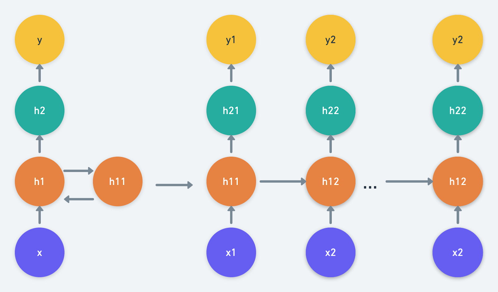
This model increases the distance traversed by a variable from time $t$ to time $t + 1$. It can have simple RNNs, GRUs, or LSTMs as its hidden units. It helps in modeling varying data representations by capturing the data from all ends, and enables passing multiple/single hidden state(s) to the multiple hidden states of the subsequent layers.

The Mathematical Notion

The hidden state in a deep RNN can be given by the following equation:

$$H^{l}_t = \phi^{l}(H^{l}_{t-1} * W^{l}_{hh} + H^{l-1}_{t} * W^{l}_{xh} + b^{l}_{h})$$

Where $\phi$ is the activation function, $W$ is the weight matrix, and $b$ is the bias.

The output at a hidden state $H_t$ is given by:

$$O_t = H^{l}_{t}  * W_{hy} + b_y$$

The training of a deep RNN is similar to the Backpropagation Through Time (BPTT) algorithm, as in an RNN but with additional hidden units.

Now that you’ve got an idea of what a deep RNN is, in the next section we'll build a music generator using a deep RNN and Keras.

Generating Music Using a Deep RNN

Music is the ultimate language. We have been creating and rendering beautiful melodies since time unknown. In this context, do you think a computer can generate musical notes comparable to how we (and a set of musical instruments) can?

Fortunately, by learning from the multitude of already existing compositions, a neural network does have the ability to generate a new kind of music. Generating music using computers is an exciting application of what a neural network can do. Music created by a neural network has both harmony and melody, and can even be passable as a human composition.

Before directly jumping into the code, let's first gain an understanding of the music representation that shall be harnessed to train the network.

Musical Instrument Digital Interface (MIDI)

MIDI is a series of messages that are interpreted by a MIDI instrument to render music. To meaningfully utilize the MIDI object, we shall use the music21 Python library which helps in acquiring the musical notes and understanding the musical notation.

Here’s an excerpt from a MIDI file that has been read using the music21 library:

[<music21.stream.Part 0x7fba822de4d0>,
 <music21.instrument.Piano 'Piano'>,
 <music21.instrument.Piano 'Piano'>,
 <music21.tempo.MetronomeMark Quarter=125.0>,
 <music21.key.Key of C major>,
 <music21.meter.TimeSignature 4/4>,
 <music21.chord.Chord D2 G2>,
 <music21.note.Rest rest>,
 <music21.chord.Chord G2 D2>,
 <music21.note.Rest rest>,
 <music21.note.Note C>,
 <music21.note.Rest rest>,
 <music21.chord.Chord D2 G2>,
 <music21.note.Rest rest>,
 <music21.chord.Chord G2 D2>,
 <music21.note.Rest rest>,
 <music21.note.Note C>,
 <music21.note.Rest rest>,
 <music21.chord.Chord D2 G2>,
 <music21.chord.Chord G2 D2>,
 <music21.note.Rest rest>,
 <music21.note.Note C>,
 <music21.note.Rest rest>,
 <music21.chord.Chord G2 D2>]

Here:

• stream is a fundamental container for music21 objects.
• instrument defines the instrument used.
• tempo specifies the speed of an underlying beat using a text string and a number.
• note contains information about the pitch, octave, and offset of the note. Pitch is the frequency, an octave is the difference in pitches, and offset refers to the location of a note.
• chord is similar to a note object, but with multiple pitches.

We shall use the music21 library to understand the MIDI files, train an RNN, and generate music of our own.

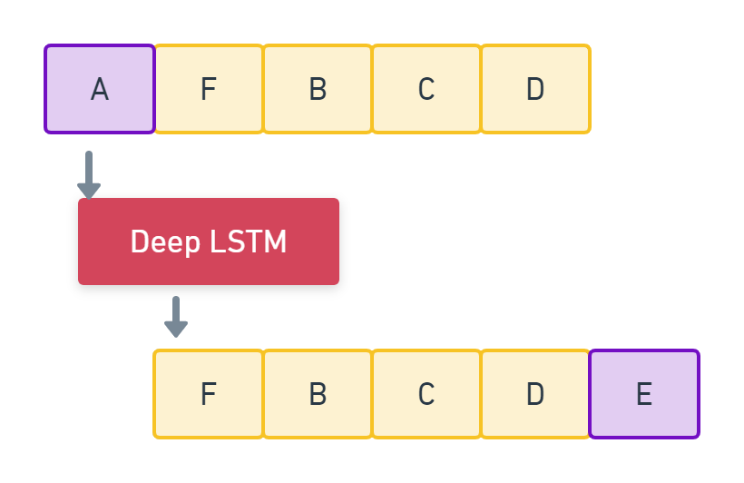
Deep LSTMs

From what you've learned so far, you can take a guess as to what kind of data music falls under. Because music is made of a series of notes, we can say that music is sequential data.

In this tutorial, we are going to use a Long Short-Term Memory (LSTM) network to remember the information for a long period of time, which is necessary for music generation. Since various musical notes and interactions have to be captured, we shall use a Deep LSTM in particular.

Step 1: Import the Dataset

First import the Groove MIDI dataset (download link) available under the Magenta project. It contains about 1,150 MIDI files and over 22,000 measures of drumming. Training on all of the data consumes a lot of time and system resources. Therefore, let’s import a small subset of the MIDI files.

To do so, use the glob.glob() method on the dataset directory to filter for .mid files.

import glob
songs = glob.glob('groovemagenta/**/*.mid', recursive=True)

Let's print the length of the dataset.

len(songs)

# Output
1150

Randomly sample 200 MIDI files from the dataset.

import random

songs = random.sample(songs, 200)
songs[:2]

# Output
['groovemagenta/groove/drummer1/session1/55_jazz_125_fill_4-4.mid',
 'groovemagenta/groove/drummer1/session1/195_reggae_78_fill_4-4.mid']

Now print the MIDI file as read by the music21 library.

!pip3 install music21

from music21 import converter

file = converter.parse(
    "groovemagenta/groove/drummer1/session1/55_jazz_125_fill_4-4.mid"
)
components = []
for element in file.recurse():
    components.append(element)

components

# Output
[<music21.stream.Part 0x7fba822de4d0>,
 <music21.instrument.Piano 'Piano'>,
 <music21.instrument.Piano 'Piano'>,
 <music21.tempo.MetronomeMark Quarter=125.0>,
 <music21.key.Key of C major>,
 <music21.meter.TimeSignature 4/4>,
 <music21.chord.Chord D2 G2>,
 <music21.note.Rest rest>,
 <music21.chord.Chord G2 D2>,
 <music21.note.Rest rest>,
 <music21.note.Note C>,
 <music21.note.Rest rest>,
 <music21.chord.Chord D2 G2>,
 <music21.note.Rest rest>,
 <music21.chord.Chord G2 D2>,
 <music21.note.Rest rest>,
 <music21.note.Note C>,
 <music21.note.Rest rest>,
 <music21.chord.Chord D2 G2>,
 <music21.chord.Chord G2 D2>,
 <music21.note.Rest rest>,
 <music21.note.Note C>,
 <music21.note.Rest rest>,
 <music21.chord.Chord G2 D2>]

Step 2: Convert MIDI to Music21 Notes

Import the required libraries.

import pickle
from music21 import instrument, note, chord, stream

Next, define a function get_notes() to fetch notes from all of the MIDI files. Load every MIDI file into a music21 stream object using the convertor.parse() method. Use this object to get all notes and chords corresponding to the MIDI file. Further, partition the music21 object in accordance with the instruments. If there’s an instrument present, check if there are any inner sub-streams available in the first part ( parts[0] ) using the recurse() method. Fetch all of the notes and chords, and append the string representation of the pitch of every note object to an array. If it’s a chord, append the id of every note to a string joined by a dot character.

""" 
Convert mid to notes
"""


def get_notes():
    notes = []

    for file in songs:
        # Convert .mid file to stream object
        midi = converter.parse(file)
        notes_to_parse = []

        try:
            # Partition stream per unique instrument
            parts = instrument.partitionByInstrument(midi)
        except:
            pass

        # If there's an instrument, enter this branch
        if parts:
            # Check if there are inner substreams available
            notes_to_parse = parts.parts[0].recurse()
        else:
            # A very important read-only property that returns a new Stream that has all
            # sub-containers “flattened” within it, that is, it returns a new Stream where
            # no elements nest within other elements.
            notes_to_parse = midi.flat.notes

        for element in notes_to_parse:
            # Extract pitch if the element is a note
            if isinstance(element, note.Note):
                notes.append(str(element.pitch))

            # Append the normal form of chord(integers) to the notes list
            elif isinstance(element, chord.Chord):
                notes.append(".".join(str(n) for n in element.normalOrder))

    with open("notes", "wb") as filepath:
        pickle.dump(notes, filepath)

    return notes

Step 3: Preprocess the Data

We have to now make our data compatible for network processing by mapping string-based to integer-based data.

First import the required libraries.

import numpy as np
from tensorflow.keras import utils

Define the sequence length (i.e. the length of an input sequence) to be 100. This means there will be 100 notes/chords in every input sequence.

Next, map music notes to integers, and create input and output sequences. Every 101st note (a note succeeding a set of 100 notes) is taken as the output for every input to train the model. Reshape the input to a 3D array: samples x timesteps x features. samples specifies the number of inputs; timesteps, the sequence length; and features, the number of outputs at every time step.

Finally, normalize the input by dividing the input with a value corresponding to the number of notes. Now convert the output to a one-hot encoded vector.

Create a function prep_seq() that maps inputs and outputs to their corresponding network-compatible data, as in the following code.

""" 
Mapping strings to real values
"""


def prep_seq(notes):

    seq_length = 100

    # Remove duplicates from the notes list
    pitchnames = sorted(set(notes))

    # A dict to map values with intgers
    notes_to_int = dict((pitch, n) for n, pitch in enumerate(pitchnames))

    net_in = []
    net_out = []

    # Iterate over the notes list by selecting 100 notes every time,
    # and the 101st will be the sequence output
    for i in range(0, len(notes) - seq_length, 1):
        seq_in = notes[i : i + seq_length]
        seq_out = notes[i + seq_length]
        net_in.append([notes_to_int[j] for j in seq_in])
        net_out.append(notes_to_int[seq_out])

    number_of_patterns = len(net_in)

    # Reshape the input into LSTM compatible (3D) which should have samples, timesteps & features
    # Samples - One sequence is one sample. A batch consists of one or more samples.
    # Time Steps - One time step is one point of observation in the sample.
    # Features - One feature is one observation at a time step.
    net_in = np.reshape(net_in, (number_of_patterns, seq_length, 1))

    # Normalize the inputs
    net_in = net_in / float(len(pitchnames))

    # Categorize the outputs to one-hot encoded vector
    net_out = utils.to_categorical(net_out)

    return (net_in, net_out)

Step 4: Define the Model

First import the required model and layers from the tensorflow.keras.models and tensorflow.keras.layers libraries, respectively.

from tensorflow.keras.models import Sequential

from tensorflow.keras.layers import (
    Activation,
    LSTM,
    Dense,
    Dropout,
    Flatten,
    BatchNormalization,
)

Moving onto the model's architecture, first define a sequential Keras block and append all of your layers to it.

The first two layers have to be LSTM blocks. The input shape of the first LSTM layer has to be the shape derived from the input data being sent to the function net_arch(). Set the number of output neurons to 256 (you can use a different number here; this certainly affects the final accuracy that you would achieve).

return_sequences in the LSTM block is set to True since the first layer's output is passed to the subsequent LSTM layer. return_sequences makes sure to maintain the shape of the data as-is, without removing the sequence length attribute, which would otherwise be ignored. recurrent_dropout is set to 0.3 to ignore 30% of the nodes used while updating the LSTM memory cells.

Next, append a BatchNormalization layer to normalize the inputs by recentering and rescaling the network data for each mini batch. This produces the regularization effect and enforces the usage of fewer training epochs, as it reduces the interdependency between layers.

Append a Dropout layer to regularize the output and prevent overfitting during the training phase. Let 0.3 be the percentage of dropout. 0.3 here means that 30% of the input neurons would be nullified.

Append a Dense layer comprised of 128 neurons, where every input node is connected to an output node.

Now add ReLU activation. Further, perform batch normalization and add dropout. Then map the previous dense layer outputs to a dense layer comprised of nodes corresponding to the number of notes. Add a softmax activation to generate the final probabilities for every note during the prediction phase.

Compile the model with categorical_crossentropy loss and adam optimizer.

Finally, define the model's architecture in a function net_arch() that accepts the model’s input data and output data length as parameters.

Add the following code to define your network architecture.

"""
Network Architecture
"""


def net_arch(net_in, n_vocab):
    model = Sequential()

    # 256 - dimensionality of the output space
    model.add(
        LSTM(
            256,
            input_shape=net_in.shape[1:],
            return_sequences=True,
            recurrent_dropout=0.3,
        )
    )
    model.add(LSTM(256))
    model.add(BatchNormalization())
    model.add(Dropout(0.3))
    model.add(Dense(128))
    model.add(Activation("relu"))
    model.add(BatchNormalization())
    model.add(Dropout(0.3))
    model.add(Dense(n_vocab))
    model.add(Activation("softmax"))

    model.compile(loss="categorical_crossentropy", optimizer="adam")
    return model

Step 5: Train Your Model

It’s always good practice to save the model’s weights during the training phase. This way you needn’t train the model again and again, each time you change something.

Add the following code to checkpoint your model's weights.

from tensorflow.keras.callbacks import ModelCheckpoint


def train(model, net_in, net_out, epochs):
    filepath = "weights.best.music3.hdf5"
    checkpoint = ModelCheckpoint(
        filepath, monitor="loss", verbose=0, save_best_only=True
    )
    model.fit(net_in, net_out, epochs=epochs, batch_size=32, callbacks=[checkpoint])

The model.fit() method is used to fit the model onto the training data, where the batch size is defined to be 32.

Fetch the music notes, prepare your data, initialize your model, define the training parameters, and call the train() method to start training your model.

epochs = 30
notes = get_notes()
n_vocab = len(set(notes))
net_in, net_out = prep_seq(notes)
model = net_arch(net_in, n_vocab)
train(model, net_in, net_out, epochs)

# Output
Epoch 1/30
2112/2112 [==============================] - 694s 329ms/step - loss: 3.5335
Epoch 2/30
2112/2112 [==============================] - 696s 330ms/step - loss: 3.2389
Epoch 3/30
2112/2112 [==============================] - 714s 338ms/step - loss: 3.2018
Epoch 4/30
2112/2112 [==============================] - 706s 334ms/step - loss: 3.1599
Epoch 5/30
2112/2112 [==============================] - 704s 333ms/step - loss: 3.0997
Epoch 6/30
2112/2112 [==============================] - 719s 340ms/step - loss: 3.0741
Epoch 7/30
2112/2112 [==============================] - 717s 339ms/step - loss: 3.0482
Epoch 8/30
2112/2112 [==============================] - 733s 347ms/step - loss: 3.0251
Epoch 9/30
2112/2112 [==============================] - 701s 332ms/step - loss: 2.9777
Epoch 10/30
2112/2112 [==============================] - 707s 335ms/step - loss: 2.9390
Epoch 11/30
2112/2112 [==============================] - 708s 335ms/step - loss: 2.8909
Epoch 12/30
2112/2112 [==============================] - 720s 341ms/step - loss: 2.8442
Epoch 13/30
2112/2112 [==============================] - 711s 337ms/step - loss: 2.8076
Epoch 14/30
2112/2112 [==============================] - 728s 345ms/step - loss: 2.7724
Epoch 15/30
2112/2112 [==============================] - 738s 350ms/step - loss: 2.7383
Epoch 16/30
2112/2112 [==============================] - 736s 349ms/step - loss: 2.7065
Epoch 17/30
2112/2112 [==============================] - 740s 350ms/step - loss: 2.6745
Epoch 18/30
2112/2112 [==============================] - 795s 376ms/step - loss: 2.6366
Epoch 19/30
2112/2112 [==============================] - 808s 383ms/step - loss: 2.6043
Epoch 20/30
2112/2112 [==============================] - 724s 343ms/step - loss: 2.5665
Epoch 21/30
2112/2112 [==============================] - 726s 344ms/step - loss: 2.5252
Epoch 22/30
2112/2112 [==============================] - 720s 341ms/step - loss: 2.4909
Epoch 23/30
2112/2112 [==============================] - 753s 357ms/step - loss: 2.4574
Epoch 24/30
2112/2112 [==============================] - 807s 382ms/step - loss: 2.4170
Epoch 25/30
2112/2112 [==============================] - 828s 392ms/step - loss: 2.3848
Epoch 26/30
2112/2112 [==============================] - 833s 394ms/step - loss: 2.3528
Epoch 27/30
2112/2112 [==============================] - 825s 391ms/step - loss: 2.3190
Epoch 28/30
2112/2112 [==============================] - 805s 381ms/step - loss: 2.2915
Epoch 29/30
2112/2112 [==============================] - 812s 384ms/step - loss: 2.2632
Epoch 30/30
2112/2112 [==============================] - 816s 386ms/step - loss: 2.2330

Step 6: Generate Predictions from the Model

This step consists of the following sub-steps:

• Fetch the already stored music notes
• Generate input sequences
• Normalize the input sequences
• Define the model by passing the new input
• Load the previous weights that were stored while training the model
• Predict the output for a randomly chosen input sequence
• Convert the output to MIDI and save it!

Create a function generate() to accommodate all of these steps.

"""
Generate a Prediction
"""


def generate():

    # Load music notes
    with open("notes", "rb") as filepath:
        notes = pickle.load(filepath)

    pitchnames = sorted(set(notes))
    n_vocab = len(pitchnames)

    print("Start music generation.")

    net_in = get_inputseq(notes, pitchnames, n_vocab)

    normalized_in = np.reshape(net_in, (len(net_in), 100, 1))
    normalized_in = normalized_in / float(n_vocab)
    model = net_arch(normalized_in, n_vocab)

    model.load_weights("weights.best.music3.hdf5")
    prediction_output = generate_notes(model, net_in, pitchnames, n_vocab)
    create_midi(prediction_output)

The get_inputseq() function returns a group of input sequences. This has already been explored in Step 3 above.

"""
Generate input sequences
"""


def get_inputseq(notes, pitchnames, n_vocab):
    note_to_int = dict((pitch, number) for number, pitch in enumerate(pitchnames))

    sequence_length = 100
    network_input = []

    for i in range(0, len(notes) - sequence_length, 1):
        sequence_in = notes[i : i + sequence_length]
        network_input.append([note_to_int[char] for char in sequence_in])

    return network_input

You can now generate 500 notes from a randomly chosen input sequence. Choose the highest probability returned by the softmax activation and reverse-map the encoded number with its corresponding note. Append the output of the already-trained character at the end of the input sequence, and start your next iteration from the subsequent character. This way we generate 500 notes by moving from one character to the next throughout the input sequence.

"""
Predict the notes from a random input sequence
"""


def generate_notes(model, net_in, notesnames, n_vocab):
    start = np.random.randint(0, len(net_in) - 1)
    int_to_note = dict((number, note) for number, note in enumerate(notesnames))
    pattern = net_in[start]
    prediction_output = []
    print("Generating notes")

    # Generate 500 notes
    for note_index in range(500):
        prediction_input = np.reshape(pattern, (1, len(pattern), 1))
        prediction_input = prediction_input / float(n_vocab)
        prediction = model.predict(prediction_input, verbose=0)

        index = np.argmax(prediction)
        result = int_to_note[index]
        prediction_output.append(result)

        # Add the generated index of the character,
        # and proceed by not considering the first char in each iteration
        pattern.append(index)
        pattern = pattern[1 : len(pattern)]

    print("Notes generated")
    return prediction_output

Finally, convert the music notes to MIDI format.

Create a function create_midi() and pass the predicted encoded output as an argument to it. Determine if the note is a note or a chord, and appropriately generate the note and chord objects respectively. If a chord, split it up into an array of notes and create a note object for every item. Append the set of notes to a chord object and an output array. If a note, simply create a note object and append it to the output array.

In the end, save the MIDI output to a test_output.mid file.

""" 
Convert the notes to MIDI format
"""


def create_midi(prediction_output):
    offset = 0
    output_notes = []

    # Create Note and Chord objects
    for pattern in prediction_output:
        # Chord
        if ("." in pattern) or pattern.isdigit():
            notes_in_chord = pattern.split(".")
            notes = []

            for current_note in notes_in_chord:
                new_note = note.Note(int(current_note))
                new_note.storedInstrument = instrument.Piano()
                notes.append(new_note)

            new_chord = chord.Chord(notes)
            new_chord.offset = offset
            output_notes.append(new_chord)
        # Note
        else:
            new_note = note.Note(pattern)
            new_note.offset = offset
            new_note.storedInstrument = instrument.Piano()
            output_notes.append(new_note)

        # Increase offset so that notes do not get clumsy
        offset += 0.5

    midi_stream = stream.Stream(output_notes)
    print("MIDI file save")
    midi_stream.write("midi", fp="test_output.mid")

Now call the generate() function.

generate()

You can play the generated mid file by uploading it into a MIDI player.

This SoundCloud tune was generated by training the model for 30 epochs on an NVIDIA K80 GPU for about 6 hours.

Conclusion

In this tutorial, you’ve learned what a Deep RNN is and how it’s preferable to a basic RNN. You’ve also trained a Deep LSTM model to generate music.

The Deep RNN (LSTM) model generated a pretty passable tune out of its learnings, though the music might seem monotonous owing to the lesser number of epochs. I would say that it's a good start!

To attain better notes and chords, I recommend you play around and modify the network's parameters. You can tune the hyperparameters, increase the number of epochs, and modify the depth of the network to check if you’re able to generate better results.

In the next part of this series, we'll be covering encoder-decoder sequence-to-sequences models.

References

Skulder Classical-Piano-Composer