Music Generation with LSTMs

Music plays a significant role in the lives of most humans. Every individual has their own taste and preference for music, whether it is pop, rock, jazz, hip hop, folk, or other such types of music. The impact of music for all of history has been revolutionary. Music, in general, can be described as a melodious and rhythmic tone that provides a soothing and calming effect to its listeners. But with all the different types of musical instruments and the variety of music, it is often a complex subject that requires humans a lot of dedication and years of effort. But how would deep learning models fare in such a complex situation?

In previous articles, we have looked at how far we have progressed in artificial intelligence and deep learning to handle numerous tasks related to audio signaling processing. Some of these audio tasks include audio classification, audio or speech recognition, audio analysis, and other similar tasks. In this blog, our primary focus is the task of music generation with the help of LSTM networks. We will understand some basic concepts and dive straight into the project. The code provided in this article can be run on the Gradient platform on Paperspace with GPU support.

Introduction:

Music generation with the help of deep learning frameworks seems like quite a complex task to accomplish. With all the different types of musical instruments and types of music, it is indeed complicated to train neural networks to generate the desired rhythmic music that might be appealing to everyone, as music is subjective. However, there are a few approaches through which we can successfully achieve this task. We will further explore this subject in the next section but first, let us understand how we can listen to audio data on your generic devices.

There are several ways in which we can listen to audio data, either through .mp3 or .wav formats. However, it is easier to gain a higher archive of data by utilizing the .midi format. MIDI files stand for Musical Instrument Digital Interface files. They can be opened with a normal VLC application or media player on an operating system. These are the type of files that are typically always used for music generation projects, and we will also use them extensively in this article.

The MIDI files do not contain any actual audio information, unlike the .mp3 or .wav formats. They contain the audio data in the form of what type of notes are to be played, the duration of how long the notes should be, and how loud the notes should be when it is played in a supportive compatible software. The primary significance of using these MIDI files is that they are compact and occupy less space. Hence, these files are perfect for music generation projects requiring large amounts of data to generate results of high quality.

Understanding Essential Concepts for Music Generation:

In one of my recent blogs, we covered audio classification with deep learning, which the viewers can check out from the following link. In that article, we understood how the data from the audio files could be converted into spectrograms, which are visual representations of the spectrum of frequencies in an audio signal. In this section of the article, our primary objective is to understand some of the more prominent methods that are mostly used for music generation.

One of the popular approaches for music generation and audio-related tasks is to use the WaveNet generative model for signal processing. This model developed by DeepMind is useful for generating raw audio data. Some of the common applications apart from generating music include the mimicking of human voices and numerous text-to-speech detection systems. Initially, this approach required a lot more computational processing power for basic tasks. However, with additional installments, most of the issues were fixed with performance improvements and are widely used in common applications. We will cover this network in perhaps a future article in more detail.

One of the other methods is to make use of 1-D convolutional layers. In 1D Convolutional layers, a convolutional operation is performed on a fixed number of filters against the input vector resulting in a single-dimensional output array. They are useful for capturing the data in input sequences and train comparatively faster than LSTMs and GRUs. However, these networks are more complex to construct because the appropriate padding selection of 'same' or 'valid' has its own issues.

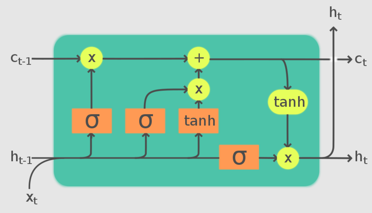
Finally, we have the LSTM method, where we develop an LSTM model that can process the task of music generation accordingly. LSTMs use a series of gates to detect which information is relevant to a particular task. From the above image, it is noticeable that these LSTM networks make use of three primary gates, namely forget, input, and output gates. One time step is completed when each of these gates is updated accordingly. In this article, we will focus on the LSTM approach for building our music generation project, as we can use these LSTM cells to construct our model architecture from scratch after some pre-processing steps.

Constructing the Music Generation Project with LSTMs:

In this section of the article, we will cover a detailed explanation of how we can generate music with the help of LSTMs. We will make use of the TensorFlow and Keras deep learning frameworks for most of the model development. You can check out the following article to learn more about TensorFlow and the Keras article here. The other essential installation that you will require for this project is the pretty midi library, which is useful for handling midi files. This library can be installed in your working environment with a simple pip command, as shown below.

pip install pretty_midi

Once we have all the necessary requirements installed in the working environment, we can start working on the music generation project. Let us get started by importing all the essential libraries.

Importing the essential libraries:

In this section, we will import all the essential libraries that are required for this project. To create the deep learning model, let us import the TensorFlow and Keras deep learning frameworks alongside all the layers, model, losses, and optimizer parameters required for the construction of the model. The other primary import is the pretty midi library, as discussed previously, to access and handle MIDI files accordingly. We will also define some libraries such as matplotlib and seaborn for the visualization of numerous parameters throughout the project. Below is the code snippet containing all the essential building blocks for the network.

import tensorflow as tf
from tensorflow.keras.layers import Input, LSTM, Dense
from tensorflow.keras.models import Model
from tensorflow.keras.losses import SparseCategoricalCrossentropy
from tensorflow.keras.optimizers import Adam

from typing import Dict, List, Optional, Sequence, Tuple
import collections
import datetime
import glob
import numpy as np
import pathlib
import pandas as pd
import pretty_midi

from IPython import display
from matplotlib import pyplot as plt
import seaborn as sns

Preparing the dataset:

The dataset we will utilize for this project will contain multiple MIDI files with numerous piano notes that our model can use for training. The MAESTRO dataset contains piano MIDI files that the viewers can download from the following link. I would recommend downloading the maestro-v2.0.0-midi.zip file. The dataset is only 57 MB in the compressed format and about 85 MB when extracted. We can use the data, which contains over 1200 files, to train and develop our deep learning model to generate music.

For most deep learning projects related to audio processing and music generation, it is usually easier to construct a deep learning architectural network to train the model for the generation of music. However, it is paramount to prepare and pre-process the data accordingly. In the next couple of sections, we will prepare and create the ideal dataset and necessary functions for training the model to produce the desired results. In the below code snippet, we are defining some essential parameters to get started with the project.

# Creating the required variables

seed = 42
tf.random.set_seed(seed)
np.random.seed(seed)

# Sampling rate for audio playback
_SAMPLING_RATE = 16000

In the next step, we will define the path to the directory where we have downloaded and extracted the data folder. The zip file, when extracted from the provided download link, should be placed in the working environment so that you can easily access all the contents present in the folder.

# Setting the path and loading the data

data_dir = pathlib.Path('maestro-v2.0.0')

filenames = glob.glob(str(data_dir/'**/*.mid*'))
print('Number of files:', len(filenames))

Once we have set the paths, we can read a sample file as shown in the code block below. By accessing a random sample file, we can gain a relatively strong understanding of how many different musical instruments are used and access some of the essential attributes required for constructing the model architecture. The three primary variables in consideration for this project are pitch, step, and duration. We can extract the necessary information by understanding the printed values of pitch, notes, and duration from the code snippet below.

# analyzing and working with a sample file

sample_file = filenames[1]
print(sample_file)

pm = pretty_midi.PrettyMIDI(sample_file)

print('Number of instruments:', len(pm.instruments))
instrument = pm.instruments[0]
instrument_name = pretty_midi.program_to_instrument_name(instrument.program)
print('Instrument name:', instrument_name)

# Extracting the notes
for i, note in enumerate(instrument.notes[:10]):
    note_name = pretty_midi.note_number_to_name(note.pitch)
    duration = note.end - note.start
    print(f'{i}: pitch={note.pitch}, note_name={note_name}, duration={duration:.4f}')

maestro-v2.0.0\2004\MIDI-Unprocessed_SMF_02_R1_2004_01-05_ORIG_MID--AUDIO_02_R1_2004_06_Track06_wav.midi
Number of instruments: 1
Instrument name: Acoustic Grand Piano
0: pitch=31, note_name=G1, duration=0.0656
1: pitch=43, note_name=G2, duration=0.0792
2: pitch=44, note_name=G#2, duration=0.0740
3: pitch=32, note_name=G#1, duration=0.0729
4: pitch=34, note_name=A#1, duration=0.0708
5: pitch=46, note_name=A#2, duration=0.0948
6: pitch=48, note_name=C3, duration=0.6260
7: pitch=36, note_name=C2, duration=0.6542
8: pitch=53, note_name=F3, duration=1.7667
9: pitch=56, note_name=G#3, duration=1.7688

The pitch values above represent the perceptual quality of sound as recognized by the MIDI note numbers. The step variable represents the time elapsed from the previous note or start of the track. Finally, the duration variable represents the difference between the start time and end time of a note, i.e., how long a particular note lasts. In the code snippet below, we extract these three parameters that will be utilized for constructing the LSTM model network to compute and generate music.

# Extracting the notes from the sample MIDI file

def midi_to_notes(midi_file: str) -> pd.DataFrame:
    pm = pretty_midi.PrettyMIDI(midi_file)
    instrument = pm.instruments[0]
    notes = collections.defaultdict(list)

    # Sort the notes by start time
    sorted_notes = sorted(instrument.notes, key=lambda note: note.start)
    prev_start = sorted_notes[0].start

    for note in sorted_notes:
        start = note.start
        end = note.end
        notes['pitch'].append(note.pitch)
        notes['start'].append(start)
        notes['end'].append(end)
        notes['step'].append(start - prev_start)
        notes['duration'].append(end - start)
        prev_start = start

    return pd.DataFrame({name: np.array(value) for name, value in notes.items()})

raw_notes = midi_to_notes(sample_file)
raw_notes.head()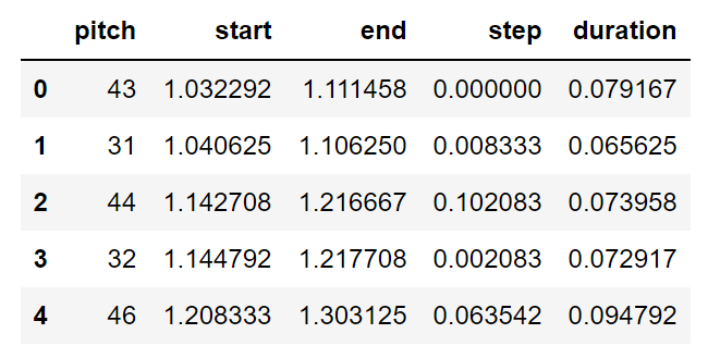

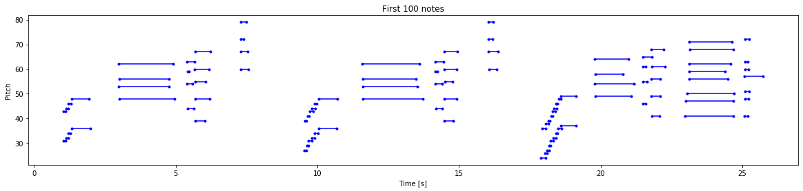
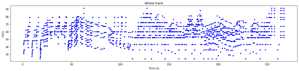
Finally, let us convert the files to vector values by using numpy arrays. We will assign numeric pitch values to note names as they are easier to interpret. The note names shown below represent the features such as note, accidental and octave number. We can also visualize our data and interpret them accordingly. Below are two visualizations: a.) Visualization of first 100 notes and b.) Visualizing the entire track.

# Converting to note names by considering the respective pitch values

get_note_names = np.vectorize(pretty_midi.note_number_to_name)
sample_note_names = get_note_names(raw_notes['pitch'])
print(sample_note_names[:10])

# Visualizing the paramaters of the muscial notes of the piano

def plot_piano_roll(notes: pd.DataFrame, count: Optional[int] = None):
    if count:
        title = f'First {count} notes'
    else:
        title = f'Whole track'
        count = len(notes['pitch'])
        
        plt.figure(figsize=(20, 4))
        plot_pitch = np.stack([notes['pitch'], notes['pitch']], axis=0)
        plot_start_stop = np.stack([notes['start'], notes['end']], axis=0)
        
        plt.plot(plot_start_stop[:, :count], plot_pitch[:, :count], color="b", marker=".")
        plt.xlabel('Time [s]')
        plt.ylabel('Pitch')
        _ = plt.title(title)

array(['G2', 'G1', 'G#2', 'G#1', 'A#2', 'A#1', 'C3', 'C2', 'F3', 'D4'],
      dtype='<U3')

Once we have finished analyzing, preparing, and visualizing our data, we can proceed to the next step to complete our pre-processing and create the final training data.

Creating the training data:

If needed, the users can also create additional data with the resources of the notes. We can generate our own MIDI files with the musical notes available. Below is the code snippet for performing the following action. Once the file is created, we can save it in the .midi format and utilize it. Hence, we can generate and create our own datasets as well if required. The generated files can be saved in the working directory or the desired location of your choice.

def notes_to_midi(notes: pd.DataFrame, out_file: str, instrument_name: str,
                  velocity: int = 100) -> pretty_midi.PrettyMIDI:

    pm = pretty_midi.PrettyMIDI()
    instrument = pretty_midi.Instrument(
      program=pretty_midi.instrument_name_to_program(
          instrument_name))

    prev_start = 0
    for i, note in notes.iterrows():
        start = float(prev_start + note['step'])
        end = float(start + note['duration'])
        
        note = pretty_midi.Note(velocity=velocity, pitch=int(note['pitch']),
                                start=start, end=end)
        instrument.notes.append(note)
        prev_start = start

    pm.instruments.append(instrument)
    pm.write(out_file)
    return pm

example_file = 'example.midi'
example_pm = notes_to_midi(
    raw_notes, out_file=example_file, instrument_name=instrument_name)

In the next step, we will focus on extracting all the notes from the MIDI files and creating our dataset. This step might be time-consuming as we have a variably large amount of data available. Depending on the type of resources that the viewers have, it is advisable to start with a few files and go from there. Below is the step to parse some amount of notes and utilize them with tf.data for higher efficiency while training and computing the model.

num_files = 5
all_notes = []
for f in filenames[:num_files]:
    notes = midi_to_notes(f)
    all_notes.append(notes)

all_notes = pd.concat(all_notes)

n_notes = len(all_notes)
print('Number of notes parsed:', n_notes)

key_order = ['pitch', 'step', 'duration']
train_notes = np.stack([all_notes[key] for key in key_order], axis=1)

notes_ds = tf.data.Dataset.from_tensor_slices(train_notes)
notes_ds.element_spec

LSTMs, as discussed previously, work best with a series of information as they are able to effectively remember the previous data elements. Hence, the dataset we create will have sequence inputs and outputs. If the size of the sequence is (100, 1), that means that there will be a total of 100 input notes that will be passed to receive a final output of 1. Therefore, the dataset we create will have a similar pattern, where the data will have notes as the input features and an output note as a label following these input sequences. Below is the code block representing the function to create these sequences.

def create_sequences(dataset: tf.data.Dataset, seq_length: int,
                     vocab_size = 128) -> tf.data.Dataset:
    """Returns TF Dataset of sequence and label examples."""
    seq_length = seq_length+1

    # Take 1 extra for the labels
    windows = dataset.window(seq_length, shift=1, stride=1,
                              drop_remainder=True)

    # `flat_map` flattens the" dataset of datasets" into a dataset of tensors
    flatten = lambda x: x.batch(seq_length, drop_remainder=True)
    sequences = windows.flat_map(flatten)

    # Normalize note pitch
    def scale_pitch(x):
        x = x/[vocab_size,1.0,1.0]
        return x

    # Split the labels
    def split_labels(sequences):
        inputs = sequences[:-1]
        labels_dense = sequences[-1]
        labels = {key:labels_dense[i] for i,key in enumerate(key_order)}

        return scale_pitch(inputs), labels

    return sequences.map(split_labels, num_parallel_calls=tf.data.AUTOTUNE)
    
seq_length = 25
vocab_size = 128
seq_ds = create_sequences(notes_ds, seq_length, vocab_size)

For selecting the sequence length, we have used 25 in the above code, but hyperparameter tuning may be used to further optimize the best sequence lengths. Finally, with the sequences created from the previous step, we can finally generate the training data by setting the batch size, buffer size, and other essential requirements for the tf.data functionality, as shown in the below code snippet.

batch_size = 64
buffer_size = n_notes - seq_length  # the number of items in the dataset
train_ds = (seq_ds
            .shuffle(buffer_size)
            .batch(batch_size, drop_remainder=True)
            .cache()
            .prefetch(tf.data.experimental.AUTOTUNE))

With the training data created successfully, we can proceed to develop our model effectively for computing and generating the music as per our requirements.

Developing the Model:

Now that we have finished preparing and processing all the essential components of the data, we can proceed to develop and train the model accordingly. The first step is to define a custom loss function that we will utilize for the step and duration parameters. We know that these parameters cannot be negative as they must always be positive integers. The function below helps to encourage the created model to only output positive values for the required parameters. Below is the code snippet for a custom mean square error loss function to perform the desired action.

def mse_with_positive_pressure(y_true: tf.Tensor, y_pred: tf.Tensor):
    mse = (y_true - y_pred) ** 2
    positive_pressure = 10 * tf.maximum(-y_pred, 0.0)
    return tf.reduce_mean(mse + positive_pressure)

Finally, we can start developing the model that we will train the dataset for generating the music. As discussed earlier, we will make use of the LSTM networks to create this model. Firstly, we will describe the input shape for the Input layer of the model. We will then call the LSTM layers with about 128 units of dimensionality space to process the data. At the end of the model network, we can define some fully connected layers for all three parameters, namely pitch, step, and duration. Once all the layers are defined, we can define the model with the input and output calls accordingly. We will use the Sparse Categorical Cross-entropy loss function for the pitch parameters while using the custom-defined mean square error loss for the step and duration parameters. We can call the Adam Optimizers and look at the summary of the model, as shown in the below code block.

# Developing the model

input_shape = (seq_length, 3)
learning_rate = 0.005

inputs = Input(input_shape)
x = LSTM(128)(inputs)

outputs = {'pitch': Dense(128, name='pitch')(x),
           'step': Dense(1, name='step')(x),
           'duration': Dense(1, name='duration')(x),
          }

model = Model(inputs, outputs)

loss = {'pitch': SparseCategoricalCrossentropy(from_logits=True),
        'step': mse_with_positive_pressure,
        'duration': mse_with_positive_pressure,
       }

optimizer = Adam(learning_rate=learning_rate)

model.compile(loss=loss, optimizer=optimizer)

model.summary()

Model: "model"
__________________________________________________________________________________________________
 Layer (type)                   Output Shape         Param #     Connected to                     
==================================================================================================
 input_1 (InputLayer)           [(None, 25, 3)]      0           []                               
                                                                                                  
 lstm (LSTM)                    (None, 128)          67584       ['input_1[0][0]']                
                                                                                                  
 duration (Dense)               (None, 1)            129         ['lstm[0][0]']                   
                                                                                                  
 pitch (Dense)                  (None, 128)          16512       ['lstm[0][0]']                   
                                                                                                  
 step (Dense)                   (None, 1)            129         ['lstm[0][0]']                   
                                                                                                  
==================================================================================================
Total params: 84,354
Trainable params: 84,354
Non-trainable params: 0
__________________________________________________________________________________________________

Once we have created the model, we can define some necessary callbacks for training the model. We will make use of the model checkpoint to save the best weights for the model, as well as define the early stopping function to terminate the program if we reach the best result and see no improvement for five epochs continuously.

# Creating the necessary callbacks

callbacks = [tf.keras.callbacks.ModelCheckpoint(filepath='./training_checkpoints/ckpt_{epoch}', save_weights_only=True),
             tf.keras.callbacks.EarlyStopping(monitor='loss', patience=5, 
                                              verbose=1, restore_best_weights=True),]

Once the model is constructed and all the necessary callbacks are defined, we can proceed to compile and fit the model accordingly. Since we have three parameters to focus on, we can compute the total loss by summing up all the losses and creating a class balance by providing specific weights to each class. We can train the model for about fifty epochs and note the type of result that is produced.

# Compiling and fitting the model

model.compile(loss = loss, 
              loss_weights = {'pitch': 0.05, 'step': 1.0, 'duration':1.0,},
              optimizer = optimizer)

epochs = 50

history = model.fit(train_ds, 
                    epochs=epochs, 
                    callbacks=callbacks,)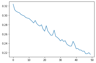

Once the model has finished training, we can analyze its performance by plotting the loss metric against the number of epochs. The reduction curve shows that the loss is constantly reducing, and the model is improving continuously. We can now proceed to look at the next step on how we can generate notes with the trained model.

Generating the notes:

Finally, we can use the trained model for generating the desired musical notes. For starting the iteration of the generation process, we will need to provide a starting sequence of notes upon which the LSTM model can continue to create building blocks and reconstruct more data elements. To create more randomness and avoid the model from picking only the best notes as it will lead to repetitive results, we can make use of the temperature parameter for random note generation. The below code snippet demonstrates the process of obtaining all the required results that we discussed in this section.

def predict_next_note(notes: np.ndarray, keras_model: tf.keras.Model, 
                      temperature: float = 1.0) -> int:
    """Generates a note IDs using a trained sequence model."""

    assert temperature > 0

    # Add batch dimension
    inputs = tf.expand_dims(notes, 0)

    predictions = model.predict(inputs)
    pitch_logits = predictions['pitch']
    step = predictions['step']
    duration = predictions['duration']

    pitch_logits /= temperature
    pitch = tf.random.categorical(pitch_logits, num_samples=1)
    pitch = tf.squeeze(pitch, axis=-1)
    duration = tf.squeeze(duration, axis=-1)
    step = tf.squeeze(step, axis=-1)

    # `step` and `duration` values should be non-negative
    step = tf.maximum(0, step)
    duration = tf.maximum(0, duration)

    return int(pitch), float(step), float(duration)

With different temperature variables and different starting sequences, we can start generating our music accordingly. The procedure for this process is demonstrated in the code block below. We make use of a random starting sequence with a random temperature value using which the LSTM model can continue to build upon. As soon as we are able to interpret the next sequence and have the required pitch, step, and duration values, we can store them in a cumulative list of generation outputs. Then, we can proceed to delete the previously used starting sequence and make use of the next preceding one to make the next prediction and store it as well. This step can be continued for a range until we have a decent tone of music generated for the desired amount of time.

temperature = 2.0
num_predictions = 120

sample_notes = np.stack([raw_notes[key] for key in key_order], axis=1)

# The initial sequence of notes while the pitch is normalized similar to training sequences
input_notes = (
    sample_notes[:seq_length] / np.array([vocab_size, 1, 1]))

generated_notes = []
prev_start = 0

for _ in range(num_predictions):
    pitch, step, duration = predict_next_note(input_notes, model, temperature)
    start = prev_start + step
    end = start + duration
    input_note = (pitch, step, duration)
    generated_notes.append((*input_note, start, end))
    input_notes = np.delete(input_notes, 0, axis=0)
    input_notes = np.append(input_notes, np.expand_dims(input_note, 0), axis=0)
    prev_start = start

generated_notes = pd.DataFrame(
    generated_notes, columns=(*key_order, 'start', 'end'))

generated_notes.head(10)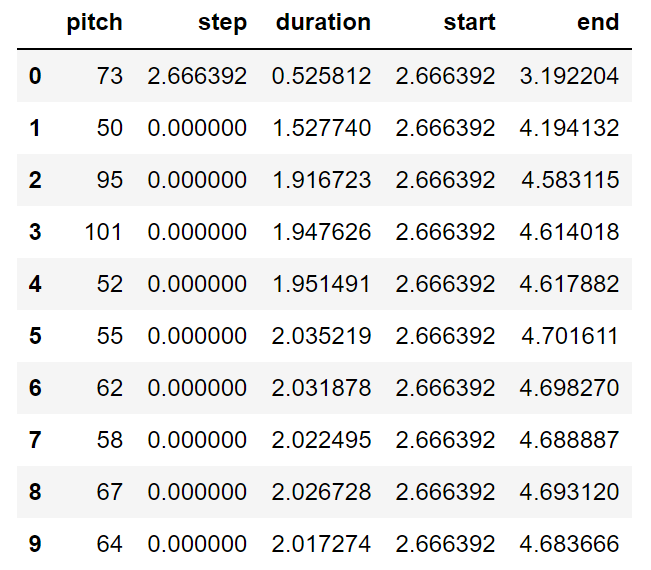

Once we have completed all the steps for music generation, we can create an output MIDI file to store the data for playing the instrument chords as generated by the model. Using our previously defined notes to midi function, we can build our MIDI file with the piano notes by using the generated outputs, mentioning the instrument type, and directing it to the output file to save the generated music notes.

out_file = 'output.midi'
out_pm = notes_to_midi(
    generated_notes, out_file=out_file, instrument_name=instrument_name)

And you can listen to a sample generated for this blog post by playing the sound file attached below.

Output

0:00

/1:04

1×

The possibilities of music generation with deep learning models are endless. There are so many different types of music genres and so many different types of networks that we can construct to achieve the desired music taste that we are looking for. The majority of the code for this article is referred to from the official TensorFlow documentation website. I would highly recommend checking out the website as well as trying out numerous different network structures and architectures to build more unique models for constructing better and more creative music generators.

Conclusion:

Music can be an integral part of most people's lives as it can create many different sorts of human emotions, like boosting memory, building task endurance, lightening your mood, reducing anxiety and depression, creating a soothing effect, and so much more. Musical instruments and music, in general, can be hard to learn, even for humans. Mastering it takes a long time as there are several different factors that one must account for and dedicate themselves to practice. However, in the modern-day, with artificial intelligence and deep learning, we have made enough progress to allow machines to step into this field and explore the nature of musical notes.

In this article, we had a brief introduction to the progress that artificial intelligence, especially deep learning models, has made in the field of music and numerous tasks related to audio and signal processing. We understood the significance of RNNs and LSTMs in creating blocks or series of data elements where the outputs can be continuously transferred to achieve outstanding results. After a quick overview of the significance of the LSTM networks, we proceeded to the next section for the construction of a music generation project from scratch. There are several improvements and advancements that can be made to the following project, and I would heavily recommend further exploration for those who are intrigued by this project.

In the upcoming articles, we will look at similar projects related to audio processing, audio recognition, and more music-related works. We will also cover concepts on neural networks from scratch and other Generative Adversarial Networks like Style GAN. Until then, enjoy exploring the world of music and deep learning networks!