
Natural Language Processing (NLP, in short) is a significant field of study. It is considered a sub-field of Artificial Intelligence, linguistics, and computer science. The capability of modern AI systems to accomplish these NLP tasks with both advanced machine learning, deep learning algorithms, and innovations has led to increasing popularity as well as overwhelming demand for accomplishing the best possible results for the following problems. One such popular task in Natural Language Processing involves finding the best solution and approach to solving the complication behind machine translation.
In this article, we will learn some of the basic elemental requirements for approaching the task of machine translation with a popular deep learning method called sequence to sequence modeling. We will dive deep into exploring the concept of RNNs, and the encoder-decoder architecture to approach this particular task. We will also study a few attention mechanisms and attempt to solve the problem of machine translation in the simplest method possible to achieve the best results.
Readers interested in only certain technical sections of the article can use the Table of Contents to read the specific topic. However, for a more concise understanding, it is preferable to cover all the concepts.
Introduction:
Machine translation is the method of utilizing Artificial Intelligence, namely deep learning mechanisms (i.e., neural network architectures), to effectively convert the translation of one language into another with relatively high accuracy and low errors (loss, in other terms). Sequence to Sequence modeling is one of the best approaches to solving tasks related to machine translation. It was one of the earlier methods that were previously used in Google Translate to obtain desirable results.
In this article, we will understand a few of the basic concepts that will help us to gain a strong intuition behind the best approach to solving problems related to machine translation. Firstly, we will go through some of the basic topics that will act as a strong starting point for the machine translation project. Before moving on to the coding section of the machine translation model architecture, I would highly recommend the viewers to check out my previous articles on TensorFlow and Keras. They will cover all the required information for approaching the coding structure of the neural network architecture.
Understanding Recurrent Neural Networks:
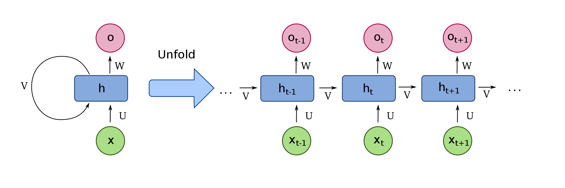
Recurrent Neural Networks (RNNs) are a popular form of artificial neural network used for a multitude of tasks such as handwriting recognition, speech synthesis, machine translation, and so much more. The term recurrent means repeating. In an RNN, the entire neural network is divided into sub neural networks and fed to the next set of sub neural networks. The image shown above is an accurate representation of how a recurrent neural network in a long sequence can potentially look like.
Recurrent Neural Networks can capture dependencies within short ranges and have the possibility to process information of any length. The RAM usage while constructing RNN model architectures is often less than the overall RAM usage in the other types of models like n-gram models. The weights are passed across through the entire set of recurrent neural networks. Hence, the computation of these networks takes into consideration all the previous data it is given. However, RNNs do suffer from a major issue because they fail to carry the relevant information for long-term dependencies because of the problem of exploding and vanishing gradients. This issue is solved by LSTMs, which we will discuss shortly.
Training Procedure
The training procedure for Recurrent Neural Networks is quite simple and can be understood by observing the figure above closely. The two steps of training, similar to most neural networks, can be divided into forwarding propagation and backpropagation. During the forward propagation, the output of the cell produced is directly equal to the type of function used (sigmoid, tanh, or other similar function) on the sum of the dot product of weights and the inputs with the previous outputs. The loss function during the forward propagation stages of each time step can be calculated as follows:

The backpropagation for the recurrent neural networks is calculated over each respective time step and not over the weights because the entire sub-networks form a complete RNN network, and each of these neural networks is actually divided into sub-networks. The representation of the backpropagation losses over each time step with respect to the weights can be computed as follows:

Brief introduction to types of RNN
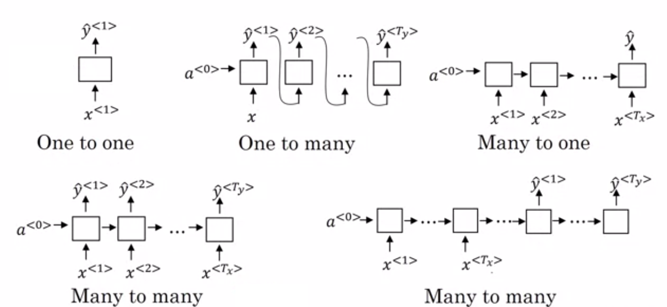
- One-to-one (Tx=Ty=1): A single input results in a single output. Typically used for a traditional neural network.
- One-to-many (Tx=1,Ty>1): Given a single input, multiple outputs are produced. A task like music generation can utilize such an RNN.
- Many-to-one (Tx>1,Ty=1): Given many inputs together produce a single output. Such RNNs find their utility in sentiment analysis.
- Many-to-many (Same Length, Tx=Ty): In this RNN, there are many inputs which give rise to many outputs but the length of the input nodes and the output nodes are equal. They are mainly used for named entity recognition.
- Many-to-many (Different Length, Tx!=Ty ): In this RNN, there are many inputs which give rise to many outputs, but the length of the input nodes and the output nodes are not equal. These types of RNNs are utilized for the task of machine translation.
Why LSTMs?
RNNs have issues with the transfer of long-term data elements due to issues of exploding and vanishing gradients. The fix to these issues is offered by the Long short-term memory (LSTM), which is also an artificial recurrent neural network (RNN) architecture that is used to solve many complex deep learning problems.
In today's project on machine translation, we will utilize these LSTMs for building our encoder-decoder architectures with a dot attention mechanism, and demonstrate how these LSTMs will lay the foundation for solving most of the recurring issues with RNNs. If you want a concise understanding of the theoretical concepts behind LSTMs, I would highly recommend checking out the part-1 article of my stock price prediction with time-series analysis.
Learning about Encoder-Decoder architectures:
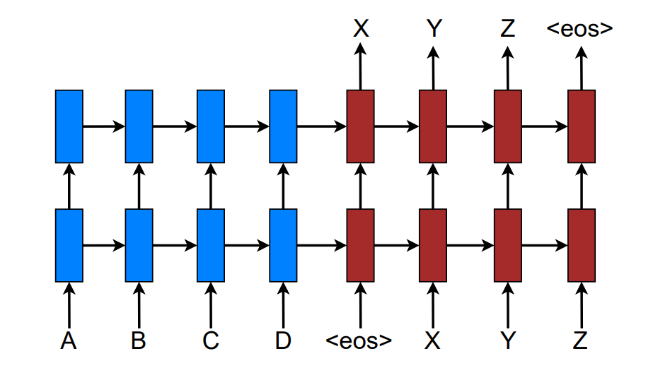
The above image representation shows a stacking recurrent architecture for translating a source sequence A B C D into a target sequence X Y Z. Here, <eos> marks the end of a sentence.
The Sequence To Sequence models usually consists of an encoder and decoder model. The encoder and decoder are two big individual components that work together to produce desirable results while performing computations. The encoder and decoder models together form the sequence-to-sequence models. The process of taking in the input sequences is done by the encoder, and the decoder has the function of producing the respective target sequences.
In the encoder, we take an input sequence associated with the particular vector. We then run this sequence of vectors through a bunch of LSTMs and store the last hidden state. Let us consider $e$ as the last hidden state encoder representation. For the decoder computations, we need to calculate the next hidden state $h0$ with the help of $e$ and the start of sentence tag $wsos$. The $s0$ is used to balance the same sizes of the vectors. We then compute the equivalent vector probabilities $p0$ with the SoftMax function. And then finally, we compute the highest probability $i0$ for the particular statement.
$$ h0 = LSTM(e,wsos) $$
$$ s0 = g(h0) $$
$$ p0 = softmax(s0) $$
$$ i0 = argmax(p0) $$
For the computation of the next stages, the repetition of these steps takes place once again. The next computation will utilize the previous hidden states and weights for the calculation of the $h1$. And the other steps remain pretty much the same.
$$ h1 = LSTM(h0,wi1) $$
$$ s1 = g(h1) $$
$$ p1 = softmax(s1) $$
$$ i1 = argmax(p1) $$
Let us now proceed to understand the significance of using attention in sequence to sequence models.
Significance of Attention:
While working with sequence to sequence models, it sometimes becomes significant to distinguish between the essential components in a particular task. I will state an example for a computer vision and NLP task. For a computer vision task, let us consider an image of a dog walking on the ground. The sequence to sequence model can identify the following fairly easily. But with the help of the attention mechanism, we can add more weightage to the essential component in the image, which is the dog. Similarly, for an NLP task, we need to focus on particular words more than others to understand the context better. Attention is useful even in these scenarios.
Let us slightly modify our previous equations to add attention to our structure and make it suitable for the sequence-to-sequence model architecture. The modified equations are as follows:
$$ht=LSTM(ht−1,[wit−1,ct])$$
$$st=g(ht)$$
$$pt=softmax(st)$$
$$it=argmax(pt)$$
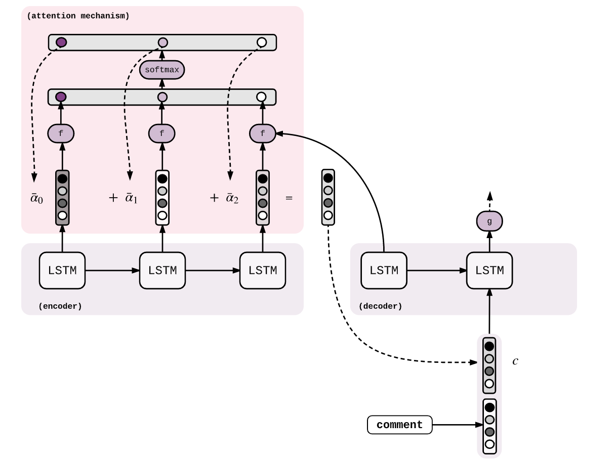
The $ct$ is the context vector utilized for processing a new context vector at each decoding step. We can compute the scores of each hidden state and then normalize the sequence with the help of the SoftMax function. And finally, we compute the weighted average.
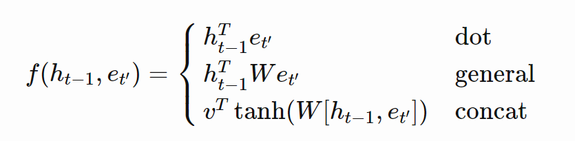
$$αt′=f(ht−1,et′)∈R $$
$$α=softmax(α)$$
$$ct=∑αt′et′$$
The type of attention can be classified with the consideration of the choice of the function. In this case, it is the $(ht−1,et′)$ component. Below is the list of the different possibilities for the attention mechanism. We will be utilizing the dot attention mechanism for the rest of the tutorial for the machine translation project.
Finally, with our basic understanding of some of the key concepts, we can practically implement our machine translation project.
Machine Translation with Sequence To Sequence Models Using Dot Attention
In this final section of the article, we will create a full working project on the implementation of machine translation with Sequence To Sequence models using dot Attention. With the help of the following link, you can implement the structure of the Bahdanau Attention. However, we will use a slightly more unique approach with the one-step decoder and the dot attention mechanism. This method will help us simplify, understand, and complete the overall project faster and better. Let us get started with the first step of the project: the dataset preparation. The Jupyter Notebooks and the dataset will be provided accordingly.
Bring this project to life
Dataset Preparation:
In the following sub-section of the article, we will look at the preparation of the dataset. The data pre-processing is a fairly straight-forward procedure, and we will try to look over this section of this article at a quick glance. The datasets for the machine translation project can be downloaded from the following website. I will utilize the Italian to English dataset for this project. I would recommend the viewers who want to follow along with the tutorial to make use of the same dataset. You can also choose to download the dataset from the attachment provided in this article.
Firstly, let us import some of the essential libraries that we will utilize for the construction of this project.
import tensorflow as tf

import matplotlib.pyplot as plt
import matplotlib.ticker as ticker
from sklearn.model_selection import train_test_split

import unicodedata
import re
import numpy as np
import os
import io
import time
Once you have completed importing all the essential libraries, it is significant to cleanse the data. Our main objective in the upcoming steps will be to remove any unnecessary information that is not required for the machine translation task. The below code block serves the purpose of opening the desired file and removing the useless data elements.
file = open("ita.txt", 'r', encoding = "utf8")
raw_data = []

for line in file:
    pos = line.find("CC-BY")
    line = line[:pos-1]

    # Split the data into english and Italian
    eng, ita = line.split('\t')

    # form tuples of the data
    data = eng, ita
    raw_data.append(data)

file.close()

def convert(list):
    return tuple(list)

data = convert(raw_data)
In the next step, we will complete the pre-processing of the dataset by removing redundant spaces and converting everything into a desirable form for simplifying the process of machine translation. We will clean the sentences by removing special characters and padding each of these sentences to a maximum specified length. Finally, we will add the <start> and <end> tokens to each of these sentences.
def unicode_to_ascii(s):
    return ''.join(
        c for c in unicodedata.normalize('NFD', s)
        if unicodedata.category(c) != 'Mn')


def preprocess_sentence(s):
    s = unicode_to_ascii(s.lower())
    s = re.sub(r'([!.?])', r' \1', s)
    s = re.sub(r'[^a-zA-Z.!?]+', r' ', s)
    s = re.sub(r'\s+', r' ', s)

    s = s.strip()
    s = '<start>' +' '+ s +' '+' <end>'
    return s
We will limit the dataset to 30000 sentences for the machine translation process. I am doing this to reduce the number of resources spent and complete the process of machine translation faster at a small cost of accuracy. However, if you have sufficient resources or more time, I would recommend using the complete dataset to achieve overall better results.
# Limiting the data and Splitting into seperate lists and add tokens

data = data[:30000]

lang_eng = []
lang_ita = []

raw_data_en, raw_data_ita = list(zip(*data))
raw_data_en, raw_data_ita = list(raw_data_en), list(raw_data_ita)

for i, j in zip(raw_data_en, raw_data_ita):
  preprocessed_data_en = preprocess_sentence(i)
  preprocessed_data_ita = preprocess_sentence(j)
  lang_eng.append(preprocessed_data_en)
  lang_ita.append(preprocessed_data_ita)

def tokenize(lang):
  lang_tokenizer = tf.keras.preprocessing.text.Tokenizer(
      filters='')
  lang_tokenizer.fit_on_texts(lang)

  tensor = lang_tokenizer.texts_to_sequences(lang)

  tensor = tf.keras.preprocessing.sequence.pad_sequences(tensor,
                                                         padding='post')

  return tensor, lang_tokenizer

input_tensor, inp_lang = tokenize(lang_ita)
target_tensor, targ_lang = tokenize(lang_eng)

max_length_targ, max_length_inp = target_tensor.shape[1], input_tensor.shape[1]
In the next code block, we will split the dataset accordingly into training and testing data. The ratio of splitting will be in the form of 80:20. Out of the 30000 data elements, we will have 24000 training elements with their respective targets and 6000 testing elements with their respective target predictions. Finally, we will map the words to some index values as a means for representing each of these values.
# Creating training and validation sets using an 80-20 split
input_tensor_train, input_tensor_val, target_tensor_train, target_tensor_val = train_test_split(input_tensor, target_tensor, test_size=0.2)

# Show length
print(len(input_tensor_train), len(target_tensor_train), len(input_tensor_val), len(target_tensor_val))

def convert(lang, tensor):
  for t in tensor:
    if t!=0:
      print ("%d ----> %s" % (t, lang.index_word[t]))

print ("Input Language; index to word mapping")
convert(inp_lang, input_tensor_train[0])
print ()
print ("Target Language; index to word mapping")
convert(targ_lang, target_tensor_train[0])
Result:
24000 24000 6000 6000
Input Language; index to word mapping
1 ----> <start>
12 ----> la
205 ----> prendero
3 ----> .
2 ----> <end>

Target Language; index to word mapping
1 ----> <start>
4 ----> i
20 ----> ll
43 ----> get
7 ----> it
3 ----> .
2 ----> <end>
We will then proceed to define a few parameters that will be useful for the training procedure and the overall preparation of the dataset.
BUFFER_SIZE = len(input_tensor_train)
BATCH_SIZE = 64
steps_per_epoch = len(input_tensor_train)//BATCH_SIZE

vocab_inp_size = len(inp_lang.word_index)+1
vocab_tar_size = len(targ_lang.word_index)+1

dataset = tf.data.Dataset.from_tensor_slices((input_tensor_train, target_tensor_train)).shuffle(BUFFER_SIZE)
dataset = dataset.batch(BATCH_SIZE, drop_remainder=True)

dataset
Once we have completed the data pre-processing step, we can move on to build our neural network architecture, starting with the Encoder structure. The encoder will contain the required LSTMs structures and embeddings, as discussed in the previous sections for a complete neural network build. Before proceeding to further coding sections, I would highly recommend checking out the TensorFlow and Keras articles respectively, to gauge more analytical and critical thinking for the upcoming code blocks.
Encoder Architecture:
We will implement the model subclassing methods for all the models from here on. Our approach for the encoder architecture is to use the main class Encoder. Then, we will utilize a couple of functions, namely the __init__ function, the initialize states block, and the call blocks. In the init block, we will define and initialize all the required parameters.
In the call block of the encoder, we define a function such that it takes an input sequence and the initial states of the encoder. The input of the input sequences is passed through the embedding layer, and finally, the output of the embedding layer is passed into the Encoder LSTM. The call function returns all the outputs of the encoder as well as the last time steps of the hidden and cell states.
The final function of the initialize states is used to represent the initialization of the hidden states and initial cell states accordingly with respect to the batch size assigned to it. A batch size of 64 will result in a Hidden state shape of [64,lstm_units] and the cell state shape of [64,lstm_units]. Let us look at the code block below for a more clear picture of the actions that are to be performed.
class Encoder(tf.keras.Model):

    def __init__(self, inp_vocab_size, embedding_size, lstm_size, input_length):
        super(Encoder, self).__init__()

        #Initialize Embedding layer
        #Intialize Encoder LSTM layer

        self.lstm_size = lstm_size
        self.embedding = tf.keras.layers.Embedding(inp_vocab_size, embedding_size)
        self.lstm = tf.keras.layers.LSTM(lstm_size, return_sequences=True, return_state=True)

    def call(self, input_sequence, states):

        embed = self.embedding(input_sequence)
        output, state_h, state_c = self.lstm(embed, initial_state=states)

        return output, state_h, state_c

    def initialize_states(self,batch_size):

        return (tf.zeros([batch_size, self.lstm_size]),
                tf.zeros([batch_size, self.lstm_size]))
Dot Attention Mechanism:
With the completion of the encoder architecture, we will proceed to look at the dot attention mechanism that will be implemented in our project. This attention method is one of the simplest approaches. However, you can choose to interpret your project with the help of other methods as well if you choose to do so. I have also provided an example code line that is commented on for the general dot attention mechanism.
For a more intuitive understanding of the code block that is represented below, let us determine some of the essential features and characteristics to understand the methodology being implemented. The Attention class is used to operate on the provided scoring function. In this case, we are making use of the dot attention mechanism. The first function in the Attention Class is used to initialize the scoring function and prepare the call function for the dot attention procedure.
In the call function, the Attention mechanism takes mainly two inputs for the current step. These two variables include the hidden states of the decoder and all the outputs of the encoder. Based on the scoring function, in this case, the dot attention mechanism, we will find the score or similarity between the hidden states of the decoder and the encoder outputs. We will then proceed to multiply the score function with the encoder outputs to get the context vector. This function will finally return the context vector and attention weights (i.e., SoftMax - scores).
class Attention(tf.keras.layers.Layer):
    def __init__(self,scoring_function, att_units):
        super(Attention, self).__init__()

        self.scoring_function = scoring_function
        self.att_units = att_units

        if self.scoring_function=='dot':
            pass
            # For general, it would be self.wa = tf.keras.layers.Dense(att_units)


    def call(self,decoder_hidden_state,encoder_output):

        if self.scoring_function == 'dot':

            new_state = tf.expand_dims(decoder_hidden_state, -1)
            score = tf.matmul(encoder_output, new_state)
            weights = tf.nn.softmax(score, axis=1)
            context = weights * encoder_output
            context_vector = tf.reduce_sum(context, axis=1)

            return context_vector, weights
One Step Decoder:
In the one-step decoder of this machine translation project, we will initialize the decoder embedding layer, LSTMs, and any other objects required. The one-step decoder is modified in such a way that it will return the necessary weights. Let us systematically understand the procedure of the one-step decoder by breaking the procedure of its implementation down into six essential steps. These are as follows:
- Pass the input_to_decoder to the embedding layer and then get the output(1,1,embedding_dim).
- Using the encoder_output and decoder hidden state, compute the context vector.
- Concatenate the context vector with the step-1 output.
- Pass the Step-3 output to LSTM/GRU and get the decoder output and states(hidden and cell state).
- Pass the decoder output to dense layer(vocab size) and store the result into output.
- Return the states from step-4, output from Step-5, attention weights from Step -2.
class One_Step_Decoder(tf.keras.Model):
    def __init__(self, tar_vocab_size, embedding_dim, input_length, dec_units, score_fun, att_units):
        super(One_Step_Decoder, self).__init__()
        # Initialize decoder embedding layer, LSTM and any other objects needed
        self.tar_vocab_size = tar_vocab_size
        self.embedding_dim = embedding_dim
        self.input_length = input_length
        self.dec_units = dec_units
        self.score_fun = score_fun
        self.att_units = att_units
        self.embedding = tf.keras.layers.Embedding(self.tar_vocab_size, self.embedding_dim,
                                                   input_length=self.input_length)

        self.lstm = tf.keras.layers.LSTM(self.dec_units, return_sequences=True,
                                         return_state=True)

        self.output_layer = tf.keras.layers.Dense(self.tar_vocab_size)

        self.attention = Attention(self.score_fun, self.att_units)

    def call(self, input_to_decoder, encoder_output, state_h, state_c):

        result = self.embedding(input_to_decoder)

        context_vector, weights = self.attention(state_h, encoder_output)

        concat = tf.concat([tf.expand_dims(context_vector, 1), result], axis=-1)

        decoder_output, hidden_state, cell_state = self.lstm(concat, initial_state=[state_h, state_c])

        final_output = tf.reshape(decoder_output, (-1, decoder_output.shape[2]))
        final_output = self.output_layer(final_output)

        return final_output, hidden_state, cell_state, weights, context_vector
Decoder Architecture:
The decoder architecture is constructed in the upcoming code block. The procedure involves initializing an empty Tensor array that will store the outputs at each and every time step. Create a tensor array as shown in the reference code block and then proceed to iterate till the length of the decoder input. Once you call the one-step decoder for each token in the decoder_input, you can proceed to store the output in the defined variable for the Tensor array. Finally, make sure that you return this tensor array.
class Decoder(tf.keras.Model):
    def __init__(self, out_vocab_size, embedding_dim, output_length, dec_units ,score_fun ,att_units):
        #Intialize necessary variables and create an object from the class onestepdecoder
        super(Decoder, self).__init__()
        self.out_vocab_size = out_vocab_size
        self.embedding_dim = embedding_dim
        self.output_length = output_length
        self.dec_units = dec_units
        self.score_fun = score_fun
        self.att_units = att_units
        self.onestepdecoder = One_Step_Decoder(self.out_vocab_size, self.embedding_dim, self.output_length,
                                               self.dec_units, self.score_fun, self.att_units)

    def call(self, input_to_decoder,encoder_output,decoder_hidden_state,decoder_cell_state):

        all_outputs= tf.TensorArray(tf.float32, size=input_to_decoder.shape[1], name="output_arrays")


        for timestep in range(input_to_decoder.shape[1]):
            output, decoder_hidden_state, decoder_cell_state, weights, context_vector = self.onestepdecoder(
                                                                                    input_to_decoder[:,timestep:timestep+1],
                                                                                    encoder_output,
                                                                                    decoder_hidden_state,
                                                                                    decoder_cell_state)

            all_outputs = all_outputs.write(timestep, output)

        all_outputs = tf.transpose(all_outputs.stack(), (1, 0, 2))

        return all_outputs
Call The Encoder Decoder Architecture:
The encoder_decoder class is an additional element to our project to simplify the overall process and combine both the elements of the encoder and decoder. In this class, we will define all the variables required for this step. The init block will consist of the initializations of the encoder and decoder blocks. The call function is used to send but mostly obtain significant information from all the other classes.
class encoder_decoder(tf.keras.Model):
    def __init__(self, inp_vocab_size, out_vocab_size, embedding_size, lstm_size,
                 input_length, output_length, dec_units ,score_fun ,att_units, batch_size):

        super(encoder_decoder, self).__init__()

        self.encoder = Encoder(inp_vocab_size, embedding_size, lstm_size, input_length)
        self.decoder = Decoder(out_vocab_size, embedding_size, output_length,
                               dec_units, score_fun, att_units)

    def call(self, data):

        input_sequence, input_to_decoder = data[0],data[1]
        initial_state = self.encoder.initialize_states(batch_size=64)
        encoder_output, state_h, state_c = self.encoder(input_sequence, initial_state)
        decoder_hidden_state = state_h
        decoder_cell_state = state_c
        decoder_output = self.decoder(input_to_decoder, encoder_output, decoder_hidden_state, decoder_cell_state)

        return decoder_output
Custom Loss Function:
After the completion of the architectural build for our machine translation model, we need to define a few parameters that are required for the process of training the model. We will make use of the Adam optimizer and utilize the loss object as the Sparse Categorical Cross-entropy for computing the cross-entropy loss between the labels and predictions. The below code block is a simple representation of how such an action can be performed. You can feel free to try out other methods or optimizers to see which suits your model the best.
loss_object = tf.keras.losses.SparseCategoricalCrossentropy(
    from_logits=True, reduction='none')

def loss_function(real, pred):
  mask = tf.math.logical_not(tf.math.equal(real, 0))
  loss_ = loss_object(real, pred)

  mask = tf.cast(mask, dtype=loss_.dtype)
  loss_ *= mask

  return tf.reduce_mean(loss_)

optimizer = tf.keras.optimizers.Adam()
Training:
The next few code blocks will deal with the implementation of the training for the Sequence To Sequence models using dot Attention. The first code block consists of only some of the initializations as well as the required library calls for the overall computation of the following training process. I was making use of Paperspace Gradient for the implementation of the machine translation project due to some GPU limitations on my system. Henceforth, I used the !mkdir logs command to create an additional directory. If you are building this model architecture on your PC, you can skip this step or directly create a folder/directory in your system.
To discuss a few more steps in the code block, we are activating the callbacks with the help of the TensorFlow and Keras deep learning frameworks. The checkpoint is the more significant callback because it will enable you to save the best weights after training, and you can export this saved model for future instances. This saved file can be used by your prediction model to make the required translations. We have also defined some of the essential variables with some desirable values for passing them to the previously defined encoder-decoder architecture.
!mkdir logs

from tensorflow.keras.callbacks import ModelCheckpoint
from tensorflow.keras.callbacks import TensorBoard

checkpoint = ModelCheckpoint("dot.h5", monitor='val_loss', verbose=1, save_weights_only=True)

logdir='logs'
tensorboard_Visualization = TensorBoard(log_dir=logdir)

input_vocab_size = len(inp_lang.word_index)+1
output_vocab_size = len(targ_lang.word_index)+1

input_len = max_length_inp
output_len = max_length_targ

lstm_size = 128
att_units = 256
dec_units = 128
embedding_size = 300
embedding_dim = 300
score_fun = 'dot'
steps = len(input_tensor)//64
batch_size=64

model = encoder_decoder(input_vocab_size,output_vocab_size,embedding_size,lstm_size,input_len,output_len,dec_units,score_fun,att_units, batch_size)

checkpoint_dir = './training_checkpoints'
checkpoint_prefix = os.path.join(checkpoint_dir, "ckpt")
checkpoint = tf.train.Checkpoint(optimizer=optimizer,
                                 encoder=model.layers[0],
                                 decoder=model.layers[1])
In the next step, we will use the teacher forcing method to train the model architecture accordingly. The gradient tape method is often used for training complex structures more easily. I would highly recommend checking out my previous article on TensorFlow to understand the functioning of the steps more appropriately. For the execution of the below code block, all the steps for the dataset preparation must be followed as described previously. For example, if the decoder input is "<start> Hi how are you", then the decoder output should be "Hi How are you <end>".
@tf.function
def train_step(inp, targ, enc_hidden):
  loss = 0

  with tf.GradientTape() as tape:
    enc_output, enc_hidden,enc_state = model.layers[0](inp, enc_hidden)


    dec_input = tf.expand_dims([targ_lang.word_index['<start>']] * BATCH_SIZE, 1)

    for t in range(1, targ.shape[1]):
      predictions = model.layers[1](dec_input,enc_output,enc_hidden,enc_state)

      loss += loss_function(targ[:, t], predictions)

      dec_input = tf.expand_dims(targ[:, t], 1)

  batch_loss = (loss / int(targ.shape[1]))

  variables = model.layers[0].trainable_variables + model.layers[1].trainable_variables

  gradients = tape.gradient(loss, variables)

  optimizer.apply_gradients(zip(gradients, variables))

  return batch_loss
We will implement our training procedure for a total of twenty epochs. You can follow the code block provided below for the following implementation. Let us proceed to look at some of the results that are obtained upon training the machine translation model.
EPOCHS = 20

for epoch in range(EPOCHS):
  start = time.time()

  enc_hidden = model.layers[0].initialize_states(64)
  total_loss = 0

  for (batch, (inp, targ)) in enumerate(dataset.take(steps_per_epoch)):
    batch_loss = train_step(inp, targ, enc_hidden)
    total_loss += batch_loss

    if batch % 100 == 0:
      print('Epoch {} Batch {} Loss {:.4f}'.format(epoch + 1,
                                                   batch,
                                                   batch_loss.numpy()))

  if (epoch + 1) % 2 == 0:
    checkpoint.save(file_prefix = checkpoint_prefix)

  print('Epoch {} Loss {:.4f}'.format(epoch + 1,
                                      total_loss / steps_per_epoch))
  print('Time taken for 1 epoch {} sec\n'.format(time.time() - start))
Result:
Epoch 18 Batch 0 Loss 0.2368
Epoch 18 Batch 100 Loss 0.2204
Epoch 18 Batch 200 Loss 0.1832
Epoch 18 Batch 300 Loss 0.1774
Epoch 18 Loss 0.1988
Time taken for 1 epoch 12.785019397735596 sec

Epoch 19 Batch 0 Loss 0.1525
Epoch 19 Batch 100 Loss 0.1972
Epoch 19 Batch 200 Loss 0.1409
Epoch 19 Batch 300 Loss 0.1615
Epoch 19 Loss 0.1663
Time taken for 1 epoch 12.698532104492188 sec

Epoch 20 Batch 0 Loss 0.1523
Epoch 20 Batch 100 Loss 0.1319
Epoch 20 Batch 200 Loss 0.1958
Epoch 20 Batch 300 Loss 0.1000
Epoch 20 Loss 0.1410
Time taken for 1 epoch 12.844841480255127 sec
We can observe that during the final few epochs, the loss has drastically reduced from its initial observations. The model has been trained well with a gradually reducing loss and an overall improvement in the accuracy of predictions. If you have the time, patience, and resources, it is recommended that you try to implement the machine translation training procedure on the entire dataset for a higher number of epochs.
Translate:
The final step of our project is to make the essential predictions. The translation procedure is completed in the predict function as shown in the below code block. The main steps are to take the given input sentence and then convert the sentence into integers using the previously defined tokenizers. Then we pass the input sequence to the encoder to receive the encoder outputs, the last time step of the hidden and the cell state as described previously. The other steps like Initializing the index of as input to decoder and encoder final states as input states to the one-step decoder are also completed in this step.
def predict(input_sentence):

  attention_plot = np.zeros((output_len, input_len))

  input_sentence = preprocess_sentence(input_sentence)

  inputs = [inp_lang.word_index[i] for i in input_sentence.split()]
  inputs = tf.keras.preprocessing.sequence.pad_sequences([inputs],
                                                         maxlen=input_len,
                                                         padding='post')
  inputs = tf.convert_to_tensor(inputs)

  result = ''

  encoder_output,state_h,state_c = model.layers[0](inputs,[tf.zeros((1, lstm_size)),tf.zeros((1, lstm_size))])

  dec_input = tf.expand_dims([targ_lang.word_index['<start>']], 0)

  for t in range(output_len):
   predictions,state_h,state_c,attention_weights,context_vector = model.layers[1].onestepdecoder(dec_input,
                                                                                                 encoder_output,
                                                                                                 state_h,
                                                                                                 state_c)

   attention_weights = tf.reshape(attention_weights, (-1, ))
   attention_plot[t] = attention_weights.numpy()

   predicted_id = tf.argmax(predictions[0]).numpy()

   result += targ_lang.index_word[predicted_id] + ' '

   if targ_lang.index_word[predicted_id] == '<end>':
     return result, input_sentence, attention_plot

   dec_input = tf.expand_dims([predicted_id], 0)

  return result, input_sentence, attention_plot
Let us implement a translation function that will perform the task of predicting the appropriate response from the Italian language to the English language. Note that I have not computed the BLEU score plot, which is also something the viewers can try to implement for observing the working of the machine translation model. Below is the simple function for the computation and prediction of the machine translation task.
def translate(sentence):
  result, sent, attention_plot = predict(sentence)

  print('Input: %s' % (sent))
  print('Predicted translation: {}'.format(result))
Let us quickly test the function and see if the model yields the desired results!
translate(u'ciao!')Result:
Input: <start> ciao !  <end>
Predicted translation: hello ! <end>
We have successfully constructed our machine translation model with the help of Sequence To Sequence Modeling and dot attention mechanism to achieve an overall low loss and higher accuracy of predictions.
Conclusion:

With the complete architectural build of the neural network model for performing the machine translation model, we have reached the end of this article. We covered most of the essential concepts required for a basic understanding on how you can build a machine translation deep learning model from scratch. These topics include the intuitive understanding of the working of recurrent neural networks, the encoder-decoder architecture, and the dot attention mechanism.
Finally, we built a complete project with full codes and theory for the task of machine translation. More importantly, we used a slightly unique method of the one-step decoder to solve this problem. The dataset and the complete project will be accessible within the frame of this article. Feel free to try it out and analyze the working by yourself.
In the upcoming articles, we will cover topics like transfer learning in complete depth and also work on other projects like image captioning with TensorFlow. Until then, keep exploring the world of deep learning and neural networks, and continue to build new projects!


