Advanced Recurrent Neural Networks: Bidirectional RNNs

In this tutorial we’ll cover bidirectional RNNs: how they work, the network architecture, their applications, and how to implement bidirectional RNNs using Keras.

Specifically, we'll cover:

• An overview of RNNs
• LSTM and GRU Blocks
• The need for bidirectional traversal
• Bidirectional RNNs
• Sentiment analysis using a bidirectional RNN
• Conclusion

Let's get started!

Overview of RNNs

Recurrent Neural Networks, or RNNs, are a specialized class of neural networks used to process sequential data. Sequential data can be considered a series of data points. For instance, video is sequential, as it is composed of a sequence of video frames; music is sequential, as it is a combination of a sequence of sound elements; and text is sequential, as it arises from a combination of letters. Modeling sequential data requires persisting the data learned from the previous instances. For example, if you are to predict the next argument during a debate, you must consider the previous argument put forth by the members involved in that debate. You form your argument such that it is in line with the debate flow. Likewise, an RNN learns and remembers the data so as to formulate a decision, and this is dependent on the previous learning.

Unlike a typical neural network, an RNN doesn’t cap the input or output as a set of fixed-sized vectors. It also doesn’t fix the amount of computational steps required to train a model. It instead allows us to train the model with a sequence of vectors (sequential data).

Interestingly, an RNN maintains persistence of model parameters throughout the network. It implements Parameter Sharing so as to accommodate varying lengths of the sequential data. If we are to consider separate parameters for varying data chunks, neither would it be possible to generalize the data values across the series, nor would it be computationally feasible. Generalization is with respect to repetition of values in a series. A note in a song could be present elsewhere; this needs to be captured by an RNN so as to learn the dependency persisting in the data. Thus, rather than starting from scratch at every learning point, an RNN passes learned information to the following levels.

To enable parameter sharing and information persistence, an RNN makes use of loops.

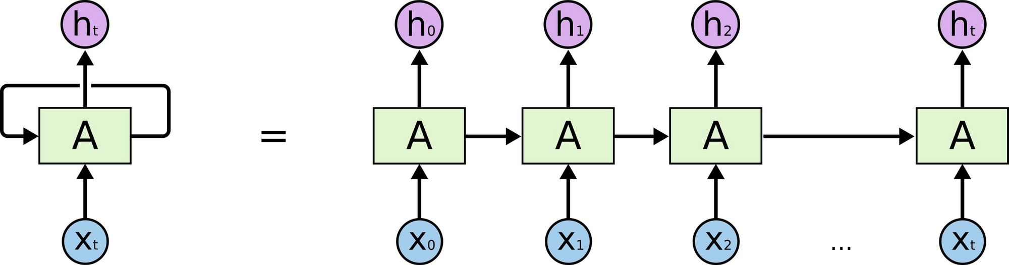
A neural network $A$ is repeated multiple times, where each chunk accepts an input $x_i$ and gives an output $h_t$. The loop here passes the information from one step to the other.

As a matter of fact, an incredible number of applications such as text generation, image captioning, speech recognition, and more are using RNNs and their variant networks.

LSTM and GRU Blocks

Not all scenarios involve learning from the immediately preceding data in a sequence. Consider a case where you are trying to predict a sentence from another sentence which was introduced a while back in a book or article. This requires remembering not just the immediately preceding data, but the earlier ones too. An RNN, owing to the parameter sharing mechanism, uses the same weights at every time step. Thus during backpropagation, the gradient either explodes or vanishes; the network doesn’t learn much from the data which is far away from the current position.

To solve this problem we use Long Short Term Memory Networks, or LSTMs. An LSTM is capable of learning long-term dependencies.

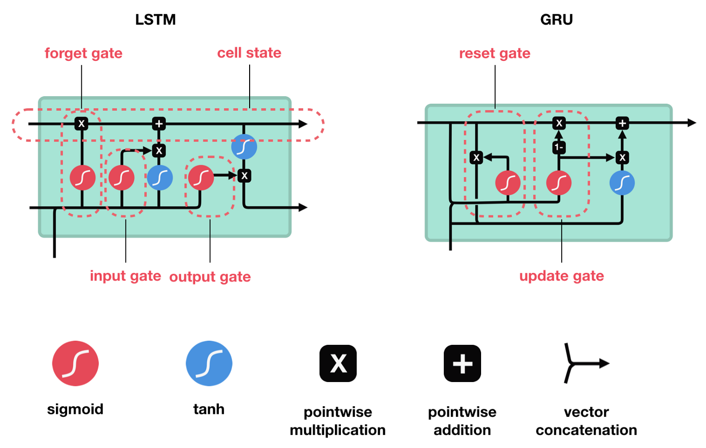
Unlike in an RNN, where there’s a simple layer in a network block, an LSTM block does some additional operations. Using input, output, and forget gates, it remembers the crucial information and forgets the unnecessary information that it learns throughout the network.

One popular variant of LSTM is Gated Recurrent Unit, or GRU, which has two gates - update and reset gates. Both LSTM and GRU work towards eliminating the long term dependency problem; the difference lies in the number of operations and the time consumed. GRU is new, speedier, and computationally inexpensive. Yet, LSTMs have outputted state-of-the-art results while solving many applications.

To learn more about how LSTMs differ from GRUs, you can refer to this article.

The Need for Bidirectional Traversal

A typical state in an RNN (simple RNN, GRU, or LSTM) relies on the past and the present events. A state at time $t$ depends on the states $x_1, x_2, …, x_{t-1}$, and $x_t$. However, there can be situations where a prediction depends on the past, present, and future events.

For example, predicting a word to be included in a sentence might require us to look into the future, i.e., a word in a sentence could depend on a future event. Such linguistic dependencies are customary in several text prediction tasks.  

Take speech recognition. When you use a voice assistant, you initially utter a few words after which the assistant interprets and responds. This interpretation may not entirely depend on the preceding words; the whole sequence of words can make sense only when the succeeding words are analyzed.

Thus, capturing and analyzing both past and future events is helpful in the above-mentioned scenarios.

Bidirectional RNNs

To enable straight (past) and reverse traversal of input (future), Bidirectional RNNs, or BRNNs, are used. A BRNN is a combination of two RNNs - one RNN moves forward, beginning from the start of the data sequence, and the other, moves backward, beginning from the end of the data sequence. The network blocks in a BRNN can either be simple RNNs, GRUs, or LSTMs.

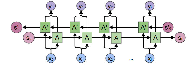
A BRNN has an additional hidden layer to accommodate the backward training process. At any given time $t$, the forward and backward hidden states are updated as follows:

$$A_t (Forward) = \phi(X_t * W_{XA}^{forward} + A_{t-1} (Forward) * W_{AA}^{forward} + b_{A}^{forward})$$

$$A_t (Backward) = \phi(X_t * W_{XA}^{backward} + A_{t+1} (Backward) * W_{AA}^{backward} + b_{A}^{backward})$$

where $\phi$ is the activation function, $W$, the weight matrix, and $b$, the bias.

The hidden state at time $t$ is given by a combination of $A_t (Forward)$ and $A_t (Backward)$. The output at any given hidden state is:

$$O_t = H_t * W_{AY} + b_{Y}$$

The training of a BRNN is similar to Back-Propagation Through Time (BPTT) algorithm. BPTT is the back-propagation algorithm used while training RNNs. A typical BPTT algorithm works as follows:

• Unroll the network and compute errors at every time step.
• Roll-up the network and update weights.

In a BRNN however, since there’s forward and backward passes happening simultaneously, updating the weights for the two processes could happen at the same point of time. This leads to erroneous results. Thus, to accommodate forward and backward passes separately, the following algorithm is used for training a BRNN:

Forward Pass

• Forward states (from $t$ = 1 to $N$) and backward states (from $t$ = $N$ to 1) are passed.
• Output neuron values are passed (from $t$ = 1 to $N$).

Backward Pass

• Output neuron values are passed ($t$ = $N$ to 1).
• Forward states (from $t$= $N$ to 1) and backward states (from $t$ = 1 to $N$) are passed.

Both the forward and backward passes together train a BRNN.

Applications

BRNN is useful for the following applications:

• Handwriting Recognition
• Speech Recognition
• Dependency Parsing
• Natural Language Processing

The bidirectional traversal idea can also be extended to 2D inputs such as images. We can have four RNNs each denoting one direction. Unlike a Convolutional Neural Network (CNN), a BRNN can assure long term dependency between the image feature maps.

Sentiment Analysis using Bidirectional RNN

Sentiment Analysis is the process of determining whether a piece of text is positive, negative, or neutral. It is widely used in social media monitoring, customer feedback and support, identification of derogatory tweets, product analysis, etc. Here we are going to build a Bidirectional RNN network to classify a sentence as either positive or negative using the sentiment-140 dataset.

You can access the cleaned subset of sentiment-140 dataset here.

Step 1 - Importing the Dataset

First, import the sentiment-140 dataset. Since sentiment-140 consists of about 1.6 million data samples, let’s only import a subset of it. The current dataset has half a million tweets.

! pip3 install wget

import wget
wget.download("https://nyc3.digitaloceanspaces.com/ml-files-distro/v1/sentiment-analysis-is-bad/data/sentiment140-subset.csv.zip")

!unzip -n sentiment140-subset.csv.zip

You now have the unzipped CSV dataset in the current repository.

Step 2 - Loading the Dataset

Install pandas library using the pip command. Later, import and read the csv file.

! pip3 install pandas
import pandas as pd

data = pd.read_csv('sentiment140-subset.csv', nrows=50000)

Step 3 - Reading the Dataset

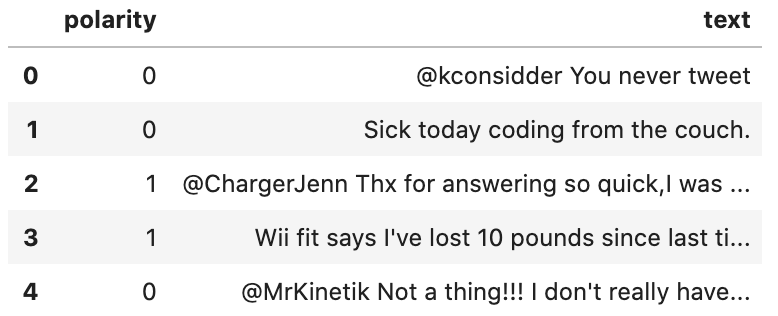
Print the data columns.

data.columns

# Output
Index(['polarity', 'text'], dtype='object')

‘Text’ indicates the sentence and ‘polarity’, the sentiment attached to a sentence. ‘Polarity’ is either 0 or 1. 0 indicates negativity and 1 indicates positivity.

Find the total number of rows in the dataset and print the first 5 rows.

print(len(data))
data.head()

# Output
50000

Step 4 - Processing the Dataset

Since raw text is difficult to process by a neural network, we have to convert it into its corresponding numeric representation.

To do so, initialize your tokenizer by setting the maximum number of words (features/tokens) that you would want to tokenize a sentence to,

import re
import tensorflow as tf

max_features = 4000

fit the tokenizer onto the text,

tokenizer = tf.keras.preprocessing.text.Tokenizer(num_words=max_features, split=' ')
tokenizer.fit_on_texts(data['text'].values)

use the resultant tokenizer to tokenize the text,

X = tokenizer.texts_to_sequences(data['text'].values)

and lastly, pad the tokenized sequences to maintain the same length across all the input sequences.

X = tf.keras.preprocessing.sequence.pad_sequences(X)

Finally, print the shape of the input vector.

X.shape

# Output
(50000, 35)

We thus created 50000 input vectors each of length 35.

Step 4 - Create a Model

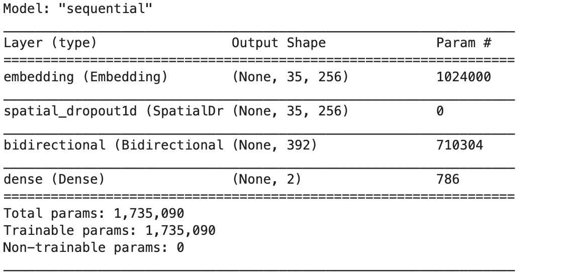
Now, let’s create a Bidirectional RNN model. Use tf.keras.Sequential() to define the model. Add Embedding, SpatialDropout, Bidirectional, and Dense layers.

• An embedding layer is the input layer that maps the words/tokenizers to a vector with embed_dim dimensions.
• The spatial dropout layer is to drop the nodes so as to prevent overfitting. 0.4 indicates the probability with which the nodes have to be dropped.
• The bidirectional layer is an RNN-LSTM layer with a size lstm_out.
• The dense is an output layer with 2 nodes (indicating positive and negative) and softmax activation function. Softmax helps in determining the probability of inclination of a text towards either positivity or negativity.

Finally, attach categorical cross entropy loss and Adam optimizer functions to the model.

embed_dim = 256
lstm_out = 196

model = tf.keras.Sequential()
model.add(tf.keras.layers.Embedding(max_features, embed_dim, input_length = X.shape[1]))
model.add(tf.keras.layers.SpatialDropout1D(0.4))
model.add(tf.keras.layers.Bidirectional(tf.keras.layers.LSTM(lstm_out, dropout=0.05, recurrent_dropout=0.2)))
model.add(tf.keras.layers.Dense(2, activation='softmax'))
model.compile(loss = 'categorical_crossentropy', optimizer='adam', metrics = ['accuracy'])

Print the model summary to understand its layer stack.

model.summary()

Step 5 - Initialize Train and Test Data

Install and import the required libraries.

import numpy as np
! pip3 install sklearn
from sklearn.model_selection import train_test_split

Create a one-hot encoded representation of the output labels using the get_dummies() method.

Y = pd.get_dummies(data['polarity'])

Map the resultant 0 and 1 values with ‘Positive’ and ‘Negative’ respectively.

result_dict = {0: 'Negative', 1: 'Positive'}
y_arr = np.vectorize(result_dict.get)(Y.columns)

y_arr variable is to be used during the model’s predictions.

Now, fetch the output labels.

Y = Y.values

Split train and test data using the train_test_split() method.

X_train, X_test, Y_train, Y_test = train_test_split(X, Y, test_size = 0.33, random_state = 42)

Print the shapes of train and test data.

print(X_train.shape, Y_train.shape)
print(X_test.shape, Y_test.shape)

# Output
(33500, 35) (33500, 2)
(16500, 35) (16500, 2)

Step 6 - Training the Model

Call the model’s fit() method to train the model on train data for about 20 epochs with a batch size of 128.

model.fit(X_train, Y_train, epochs=20, batch_size=128, verbose=2)

# Output
Train on 33500 samples
Epoch 1/20
33500/33500 - 22s - loss: 0.5422 - accuracy: 0.7204
Epoch 2/20
33500/33500 - 18s - loss: 0.4491 - accuracy: 0.7934
Epoch 3/20
33500/33500 - 18s - loss: 0.4160 - accuracy: 0.8109
Epoch 4/20
33500/33500 - 19s - loss: 0.3860 - accuracy: 0.8240
Epoch 5/20
33500/33500 - 19s - loss: 0.3579 - accuracy: 0.8387
Epoch 6/20
33500/33500 - 19s - loss: 0.3312 - accuracy: 0.8501
Epoch 7/20
33500/33500 - 18s - loss: 0.3103 - accuracy: 0.8624
Epoch 8/20
33500/33500 - 19s - loss: 0.2884 - accuracy: 0.8714
Epoch 9/20
33500/33500 - 19s - loss: 0.2678 - accuracy: 0.8813
Epoch 10/20
33500/33500 - 19s - loss: 0.2477 - accuracy: 0.8899
Epoch 11/20
33500/33500 - 19s - loss: 0.2310 - accuracy: 0.8997
Epoch 12/20
33500/33500 - 18s - loss: 0.2137 - accuracy: 0.9051
Epoch 13/20
33500/33500 - 19s - loss: 0.1937 - accuracy: 0.9169
Epoch 14/20
33500/33500 - 19s - loss: 0.1826 - accuracy: 0.9220
Epoch 15/20
33500/33500 - 19s - loss: 0.1711 - accuracy: 0.9273
Epoch 16/20
33500/33500 - 19s - loss: 0.1572 - accuracy: 0.9339
Epoch 17/20
33500/33500 - 19s - loss: 0.1448 - accuracy: 0.9400
Epoch 18/20
33500/33500 - 19s - loss: 0.1371 - accuracy: 0.9436
Epoch 19/20
33500/33500 - 18s - loss: 0.1295 - accuracy: 0.9475
Epoch 20/20
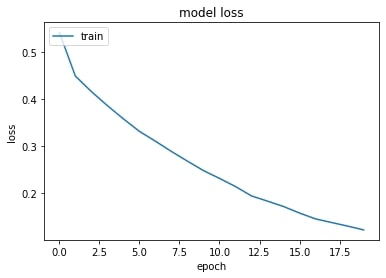
33500/33500 - 19s - loss: 0.1213 - accuracy: 0.9511

Plot accuracy and loss graphs captured during the training process.

import matplotlib.pyplot as plt

plt.plot(history.history['accuracy'])
plt.title('model accuracy')
plt.ylabel('accuracy')
plt.xlabel('epoch')
plt.legend(['train'], loc='upper left')
plt.show()

plt.plot(history.history['loss'])
plt.title('model loss')
plt.ylabel('loss')
plt.xlabel('epoch')
plt.legend(['train'], loc='upper left')
plt.show()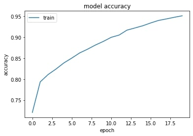

Step 7 - Computing the Accuracy

Print the prediction score and accuracy on test data.

score, acc = model.evaluate(X_test, Y_test, verbose=2, batch_size=64)
print("score: %.2f" % (score))
print("acc: %.2f" % (acc))

# Output:
16500/1 - 7s - loss: 2.0045 - accuracy: 0.7444
score: 1.70
acc: 0.74

Step 8 - Perform Sentiment Analysis

Now's the time to predict the sentiment (positivity/negativity) for a user-given sentence. First, initialize it.

twt = ['I do not recommend this product']

Next, tokenize it.

twt = tokenizer.texts_to_sequences(twt)

Pad it.

twt = tf.keras.preprocessing.sequence.pad_sequences(twt, maxlen=X.shape[1], dtype='int32', value=0)

Predict the sentiment by passing the sentence to the model we built.

sentiment = model.predict(twt, batch_size=1)[0]
print(sentiment)

if(np.argmax(sentiment) == 0):
    print(y_arr[0])
elif (np.argmax(sentiment) == 1):
    print(y_arr[1])

# Output:
[9.9999976e-01 2.4887424e-07]
Negative

The model tells us that the given sentence is negative.

Conclusion

A Bidirectional RNN is a combination of two RNNs training the network in opposite directions, one from the beginning to the end of a sequence, and the other, from the end to the beginning of a sequence. It helps in analyzing the future events by not limiting the model's learning to past and present.

In the end, we have done sentiment analysis on a subset of sentiment-140 dataset using a Bidirectional RNN.

In the next part of this series, you shall be learning about Deep Recurrent Neural Networks.

References

1. Peter Nagy
2. Colah
3. Deep Learning by Ian Goodfellow, Yoshua Bengio, and Aaron Courville