Beginner's Guide to Boltzmann Machines in PyTorch

As research progressed and researchers could bring in more evidence about the architecture of the human brain, connectionist machine learning models came into the spotlight. Connectionist models, which are also called Parallel Distributed Processing (PDP) models, are made of highly interconnected processing units. These models are generally used for complicated patterns, like human behaviour and perception. Likewise, tasks such as modelling vision, perception, or any constraint satisfaction problem need substantial computational power. The hardware support necessary for such models wasn’t previously available–that is, until the advent of VLSI technology and GPUs. This was when Boltzmann Machines were developed. In this article, we'll discuss the working of Boltzmann machines and implement them in PyTorch.

The following topics will be covered:

• The Story Behind Boltzmann Machines
• Working of Boltzmann Machines
• Intuition Behind Boltzmann Machines
• Boltzmann Machines for CSPs
• Hyperparameters
• Different Types of Boltzmann Machines
• Implementation in PyTorch

The Story Behind Boltzmann Machines

Geoffrey Hinton, sometimes referred to as the "Father of Deep Learning", formulated the Boltzmann Machine along with Terry Sejnowski, a professor at Johns Hopkins University. It is often said that Boltzmann Machines lie at the juncture of Deep Learning and Physics. These models are based on the parallel processing methodology which is widely used for dimensionality reduction, classification, regression, collaborative filtering, feature learning, and topic modelling. It is to be noted that in the Boltzmann machine’s vocabulary of building neural networks, parallelism is attributed to the parallel updation of weights of hidden layers.

Working of Boltzmann Machines

The working of Boltzmann Machine is mainly inspired by the Boltzmann Distribution which says that the current state of the system depends on the energy of the system and the temperature at which it is currently operating. Hence to implement these as Neural Networks, we use the Energy Models. The energy term was equivalent to the deviation from the actual answer. The higher the energy, the more the deviation. It has been thus important to train the model until it reaches a low-energy point. It has been obvious that such a theoretical model would suffer from the problem of local minima and result in less accurate results.

This has been solved by allowing the model to make periodic jumps to a higher energy state and then converge back to the minima, finally leading to the global minima.  We shall discuss the energy model in much greater detail in the further sections.

Let’s now see how Boltzmann Machines can be applied on two types of problems i.e., learning and searching.

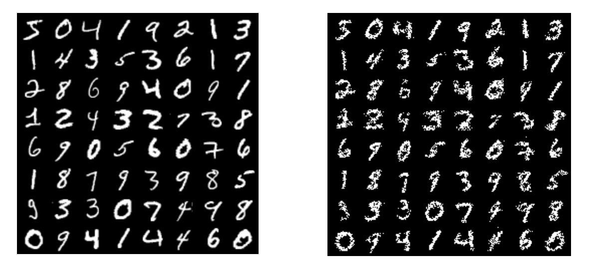
• Learning: When Boltzmann Machines are employed in learning, they try to derive important features from the input, reconstruct this input, and render it as output by parallel updation of weights. Let’s take an example by considering the MNIST dataset. The following figure shows the reconstructed output of Restricted Boltzmann Machines when applied on the MNIST dataset.

It is essential to note that during this learning and reconstruction process, Boltzmann Machines also might learn to predict or interpolate missing data. Consider working with a Movie Review dataset. Using Boltzmann Machines, we can predict whether a user will like or dislike a new movie.

• Searching: The architecture and working of Boltzmann Machines suit well to solve a constraint satisfaction problem (searching for a solution which can satisfy all constraints), even when it has weak constraints. A problem having weak constraints tries to obtain an answer which may be close enough to the answer which completely satisfies all the constraints i.e., the answer need not completely satisfy all the constraints.

In the next section, let’s look into the architecture of Boltzmann Machines in detail.

Intuition behind Boltzmann Machines

Unlike other neural network models that we have seen so far, the architecture of Boltzmann Machines is quite different. There is no clear demarcation between the input and output layer. In fact, there is no output layer. The nodes in Boltzmann Machines are simply categorized as visible and hidden nodes. The visible nodes take in the input. The same nodes which take in the input will return back the reconstructed input as the output. This is achieved through bidirectional weights which will propagate backwards and render the output on the visible nodes.

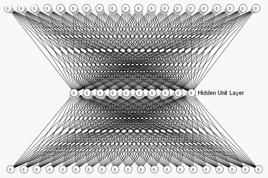
A major boost in the architecture is that every node is connected to all the other nodes, even within the same layer (for example, every visible node is connected to all the other visible nodes as well as the hidden nodes). All the links are bidirectional and the weights are symmetric. Below is an image explaining the same.

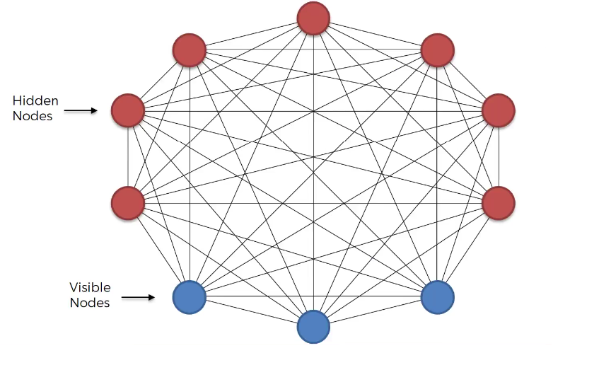
Also, every node has only two possible states i.e., on and off. The state of a node is determined by the weights and biases associated with it. The input being provided to the model i.e., the nodes (hypotheses) related directly or indirectly to that particular input will be on.

Boltzmann Machines for CSPs

As discussed earlier, the approach a Boltzmann Machine follows when dealing with a learning problem and a search problem differ.

Constraint Satisfaction Problem are in short called as CSPs

In case of a search problem, the weights on the connections are fixed and they are used to represent the cost function of an optimization problem. By utilizing a stochastic approach, the Boltzmann Machine models the binary vectors and finds optimum patterns which can be good solutions for the optimization problem. In case of a learning problem, the model tries to learn the weights to propose the state vectors as good solutions to the problem at hand. Let’s make things clear by examining how the architecture shapes itself to solve a constraint satisfaction problem (CSP).

Each node in the architecture is said to be a hypothesis and the connection between any two nodes is the constraint. If Hypothesis h1 supports Hypothesis h2, then the connection is positive. As Boltzmann Machines can solve Constraint Satisfaction Problems with weak constraints, each constraint has an importance-value associated with it. The connection weight determines how important this constraint is. If the weight is large, the constraint is more important and vice-versa. The bias applied on each node determines the likelihood of a node to be ‘on’, in case of an absence of evidence to support that hypothesis. If the bias is positive, the node is kept ‘on’, else ‘off’.

Using such a setup, the weights and states are altered as more and more examples are fed into the model; until and unless it can generate an output which satisfies most of the prioritized constraints. The training process could be stopped if a good-enough output is generated. The catch here is the output is said to be good if it leaves the model in a low-energy state. The lowest energy output will be chosen as the final output.

Hyperparameters for Boltzmann Machines

Corresponding to the other neural network architectures, hyperparameters play a critical role in training a Boltzmann Machine. Below are a few important hyperparameters that are needed to be prioritised besides the typical activation, loss, learning rate.

1. Weight Initialization: Initialization of weights is an important step in the training process. Proper initialization of weights can save a lot of time as it can optimize the time required to learn those weights, which is the whole idea of training a network. As the weights get better, the network can send better signals to make its classification results more accurate.
2. Visible and Hidden Units: The number of inputs is the feature that is explicitly given to the network. The number of hidden features has to be optimally chosen to make the network grasp a majority of features. Each of these layers has its own transform function to process the inputs and pass them onto the next layer.
3. Regularization: Through regularization, a network’s chance of overfitting is pulled away. Whenever the model overfits or learns large weights, it is penalized as it helps in reducing the weights to an acceptable level.

In the next section, let’s review different types of Boltzmann Machines.

Types of Boltzmann Machines

As discussed, Boltzmann Machine was developed to model constraint satisfaction problems which have weak constraints. But its reach has spread to solve various other problems. There are a few variations in Boltzmann Machines  which have evolved over time to solve these problems based on the use case they fall in with. Let’s review them in brief in the below sections.

Boltzmann Machines with Memory

In a conventional Boltzmann Machine, a node is aware of  all those nodes which trigger the current node at the moment. In the case of Boltzmann Machines with memory, along with the node that is responsible for the current node to get triggered, each node will know the time step at which this happens. This mechanism enables such a model to predict sequences. For example, they can be used to predict the words to auto-fill incomplete words. Say, when SCI is given as the input, there’s a possibility that the Boltzmann Machine could predict the output as SCIENCE.

In general, a memory unit is added to each unit. This alters the probability of a node being activated at any moment, depending on the previous values of other nodes and its own associated weights. This is implemented through a conduction delay about the states of nodes to the next node. On the whole, this architecture has the power to recreate training data across sequences.

Restricted Boltzmann Machines

A major complication in conventional Boltzmann Machines is the humongous number of computations despite the presence of a smaller number of nodes. In such a case, updating weights is time-taking because of dependent connections. To reduce this dependency, a restriction has been laid on these connections to restrict the model from having intra-layer connections.

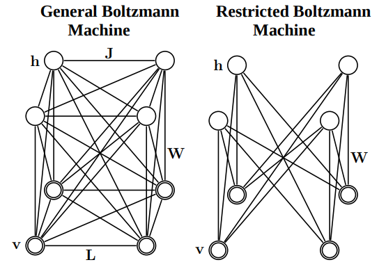
This restriction imposed on the connections made the input and the hidden nodes independent within the layer. So now, the weights could be updated parallelly.

Deep Boltzmann Machines

Deep Boltzmann Machines can be assumed to be like a stack of RBMs, which differ slightly from Deep Belief Networks. Conventional Boltzmann Machines use randomly generated Markov chains (which give the sequence of occurrence of possible events) for initialization, which are fine-tuned later as the training proceeds. This process is too slow to be practical. To combat this, Deep Boltzmann Machines follow a different approach. Their architecture is similar to Restricted Boltzmann Machines containing many layers. Each layer is pretrained greedily and then the whole model is fine-tuned through backpropagation.

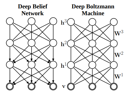
Deep Boltzmann Machines are often confused with Deep Belief networks as they work in a similar manner. The difference arises in the connections. Connections in DBNs are directed in the later layers, whereas they are undirected in DBMs.

Implementation of RBMs in PyTorch

In this section, we shall implement Restricted Boltzmann Machines in PyTorch. We shall be building a classifier using the MNIST dataset. Amongst  the wide variety of Boltzmann Machines which have already been introduced, we will be using Restricted Boltzmann Machine Architecture here. Below are the steps involved in building an RBM from scratch.

Step 1: Importing the required libraries

In this step, we import all the necessary libraries. Additionally, for the purpose of visualizing the results, we shall use torchvision.utils.

import numpy as np
import torch
import torch.utils.data
import torch.nn as nn
import torch.nn.functional as F
import torch.optim as optim
from torch.autograd import Variable
from torchvision import datasets, transforms
from torchvision.utils import make_grid , save_image
%matplotlib inline
import matplotlib.pyplot as plt

Step 2: Loading the MNIST Dataset

In this step, we will be using the MNIST Dataset using the DataLoader class of the torch.utils.data library to load our training and testing datasets. We set the batch size to 64 and apply transformations.

batch_size = 64
train_loader = torch.utils.data.DataLoader(
datasets.MNIST('./data',
    train=True,
    download = True,
    transform = transforms.Compose(
        [transforms.ToTensor()])
     ),
     batch_size=batch_size
)

test_loader = torch.utils.data.DataLoader(
datasets.MNIST('./data',
    train=False,
    transform=transforms.Compose(
    [transforms.ToTensor()])
    ),
    batch_size=batch_size)

Step 3: Defining the Model

In this step, we will start building our model. We will define the transformations associated with the visible and the hidden neurons. Also, since a Boltzmann Machine is an energy-model, we also define an energy function to calculate the energy differences. In the initialization function, we also initialize the weights and biases for the hidden and visible neurons.

class RBM(nn.Module):
   def __init__(self,
               n_vis=784,
               n_hin=500,
               k=5):
        super(RBM, self).__init__()
        self.W = nn.Parameter(torch.randn(n_hin,n_vis)*1e-2)
        self.v_bias = nn.Parameter(torch.zeros(n_vis))
        self.h_bias = nn.Parameter(torch.zeros(n_hin))
        self.k = k
    
   def sample_from_p(self,p):
       return F.relu(torch.sign(p - Variable(torch.rand(p.size()))))
    
   def v_to_h(self,v):
        p_h = F.sigmoid(F.linear(v,self.W,self.h_bias))
        sample_h = self.sample_from_p(p_h)
        return p_h,sample_h
    
   def h_to_v(self,h):
        p_v = F.sigmoid(F.linear(h,self.W.t(),self.v_bias))
        sample_v = self.sample_from_p(p_v)
        return p_v,sample_v
        
   def forward(self,v):
        pre_h1,h1 = self.v_to_h(v)
        
        h_ = h1
        for _ in range(self.k):
            pre_v_,v_ = self.h_to_v(h_)
            pre_h_,h_ = self.v_to_h(v_)
        
        return v,v_
    
   def free_energy(self,v):
        vbias_term = v.mv(self.v_bias)
        wx_b = F.linear(v,self.W,self.h_bias)
        hidden_term = wx_b.exp().add(1).log().sum(1)
        return (-hidden_term - vbias_term).mean()

As we have seen earlier, in the end, we always define the forward method which is used by the Neural Network to propagate the weights and the biases forward through the network and perform the computations. The process is repeated for k times, which defines the number of times contrastive divergence is computed. Since Boltzmann Machines are energy based machines, we now define the method which calculates the energy state of the model.

Step 4: Initialising and Training the Model

The RBM class is initialized with k as 1. We will be using the SGD optimizer in this example. At the end of the process we would accumulate all the losses in a 1D array for which we first initialize the array. We extract a Bernoulli's distribution using the data.bernoulli() method. This is the input pattern that we will start working on.

The generated pattern is next fed to the rbm model object. The model returns the pattern that it was fed and the calculated pattern as the output. The loss is calculated as the difference between the energies in these two patterns and appends it to the list. As discussed earlier, since the optimizer performs additive actions, we initially initialize the accumulators to zero. The loss is back propagated using the backward() method. optimizer.step() performs a parameter update based on the current gradient (accumulated and stored in the .grad attribute of a parameter during the backward() call) and the update rule.

rbm = RBM(k=1)
train_op = optim.SGD(rbm.parameters(),0.1)

for epoch in range(10):
    loss_ = []
    for _, (data,target) in enumerate(train_loader):
        data = Variable(data.view(-1,784))
        sample_data = data.bernoulli()
        
        v,v1 = rbm(sample_data)
        loss = rbm.free_energy(v) - rbm.free_energy(v1)
        loss_.append(loss.data)
        train_op.zero_grad()
        loss.backward()
        train_op.step()

    print("Training loss for {} epoch: {}".format(epoch, np.mean(loss_)))

In the below code snippet, we have defined a helper function in which we transpose the numpy image to suitable dimensions and store it in local storage with the name passed as an input to the function.

def show_adn_save(file_name,img):
    npimg = np.transpose(img.numpy(),(1,2,0))
    f = "./%s.png" % file_name
    plt.imshow(npimg)
    plt.imsave(f,npimg)

Step 5: Visualising the Outputs

In this step wee visualise the outputs!

show_adn_save("real",make_grid(v.view(32,1,28,28).data))

show_adn_save("generate",make_grid(v1.view(32,1,28,28).data))

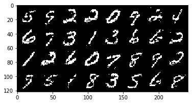
As we can see, on top we have the real image from the MNIST dataset and below is the image generated by the Boltzmann Machine.

I hope you enjoyed reading the article!