Why GANs are awesome?

When we talk about modern deep learning, the first, most popular, and often most useful concept that comes to mind is Generative Adversarial Networks (GANs). These have a lot of great applications, such as :

• Generating realistic human faces that do not exist

These faces are all fake, all made by a GAN, so sadly you can't meet them 😔.

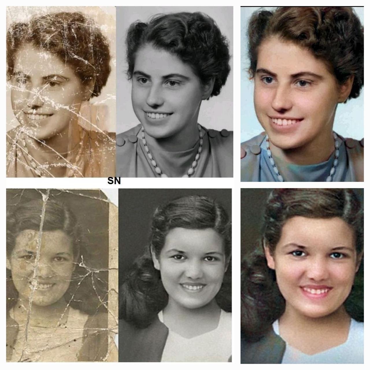
• Restoration, colonizing, and improving the resolution of photos

If you have an outdated damaged image, GANs can help you restore it, add some colors and improve its resolution😊.

Follow this tutorial on GFPGAN to learn how to upscale and restore damaged photos.

• Transforming images across domains, style transfer

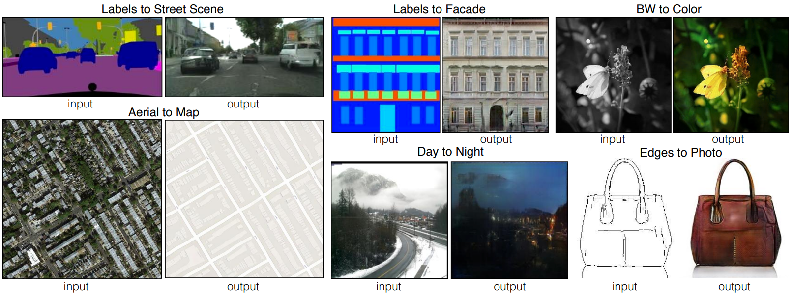
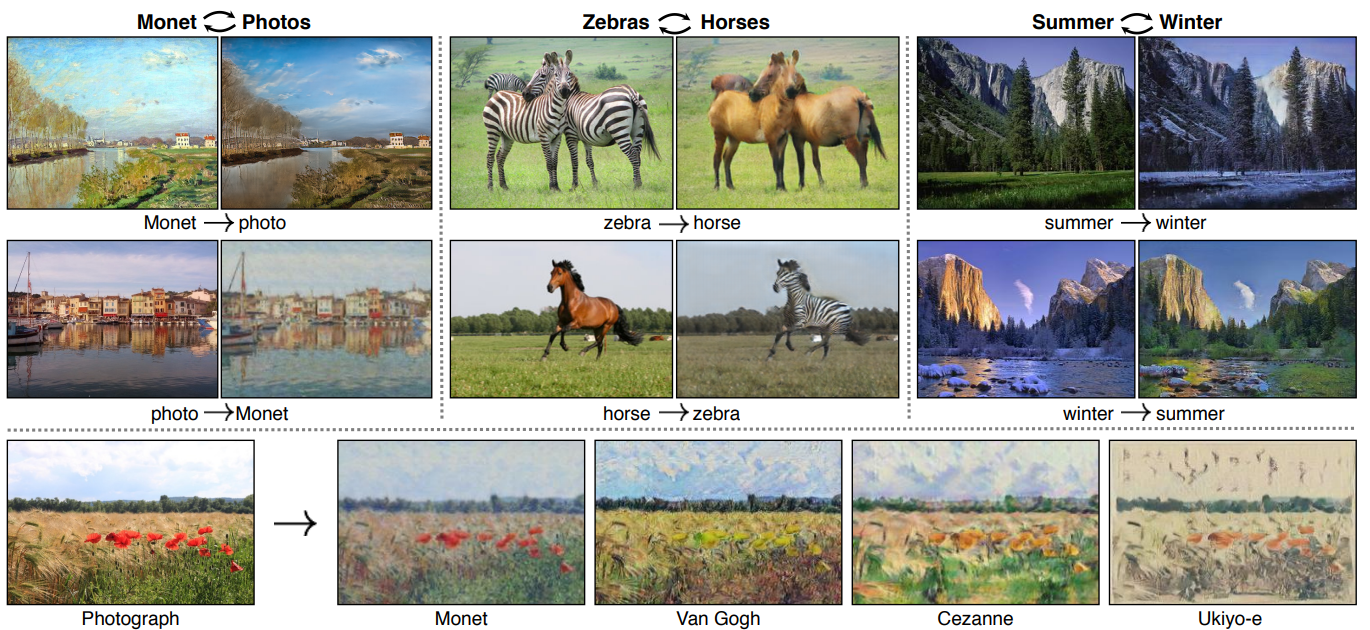
Another cool application is transforming images across domains. For example, using style transfer, we can take an image of a horse and convert it to zebra, take an image of summer and convert it into winter, or take a semantic map and output a realistic image of that semantic map.

Check out this tutorial to learn how to apply such transformations to human faces with JojoGAN.

• Data augmentation

GANs are also frequently used in data augmentation, which is a pretty clear application, but what might not be so clear is the utility of these models for medical applications. Since data from GANs doesn't come from a real person, it means that it can be used without the ethical and privacy concerns and limitations, which is a really cool application.

Summary:

What we saw until now is just a small list of examples, there are many many more. New applications are being discovered every day because it's such a hot field in research. Now let's move on to look at what GANs really are, and see the idea behind them.

What are GANs and how do they work?

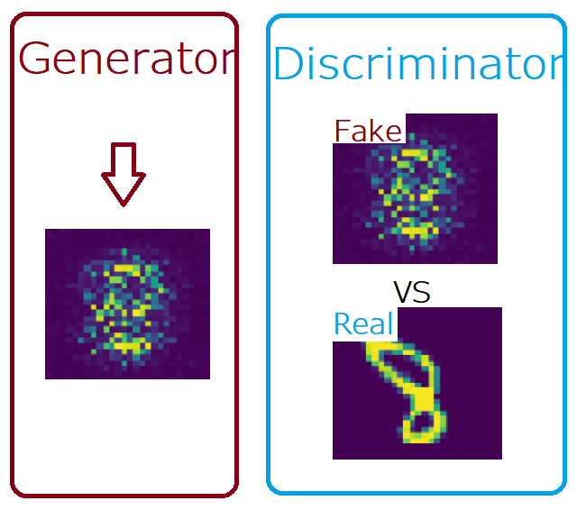
GANs are a class of machine learning techniques that consists of two networks playing an adversarial game against each other. One of these networks is called the generator, which creates the samples, and the other network is the discriminator, which attempts to discern how realistic the image is compared to a real version.

Let's say the generator wants to print a fake set of handwritten digits, and a discriminator wants to distinguish between fake and real ones. In the training process of GANs, let's say the generator is trying to print handwritten digit containing the number eight. Initially, every generated sample looks like random noise due to lack of training, and so the discriminator is going to try and compare the similarity of the generated random sample and a real image of the digit eight. In this case, it's going to say that the one coming from the generator is fake, and so the generator is not able to fool the discriminator at the start.

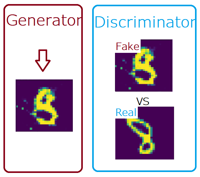
But as training goes on the generator goes on longer, it will now potentially produce something that looks close to a real handwritten eight. This is because at each step, the loss between the real and fake image is backpropogated to the start for the next iteration. Each step of gradient descent lowers the distance between the true and generated distributions, for the real and generated image respectively.

Using human insight on the example image above, we can see some incorrect pixels, so we can infer the discriminator might look at those two and say again that the one that is coming from the generator is fake. Nonetheless, progress is being made.

As training goes on even further the generator will begin to create outputs that look even more real. When the discriminator can not distinguish between the fake and real samples, it will eventually try to assert that the real handwritten digit is the fake one. Finally, the generator was able to fool the discriminator.

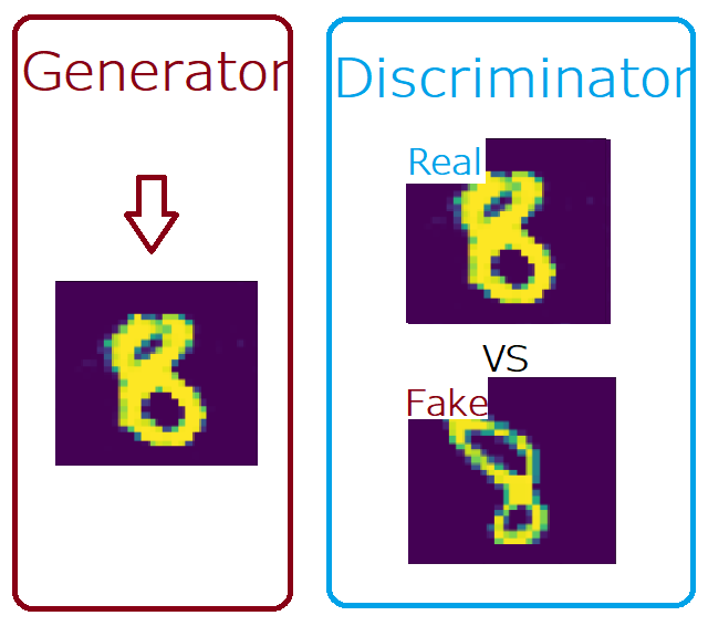
In the end, the generator generates handwritten digits virtually indistinguishable from real ones and the discriminator is forced to guess (with a rough success probability of 1/2).

Note: Both the discriminator and generator actually start from scratch meaning they are both randomly initialized at the start and then simultaneously trained.

What's the loss function?

I think now it's pretty clear that, in GANs, we have a network for the generator, and we have another network for the discriminator, and we're going to see how to implement that later.

One of the most important parts to understand right now is what the loss function looks like and how it works.

Discriminator loss

While the discriminator is trained, it classifies both the real data and the fake data from the generator.

It penalizes itself for misclassifying a real instance as fake, or a fake instance (created by the generator) as real, by maximizing the below function.

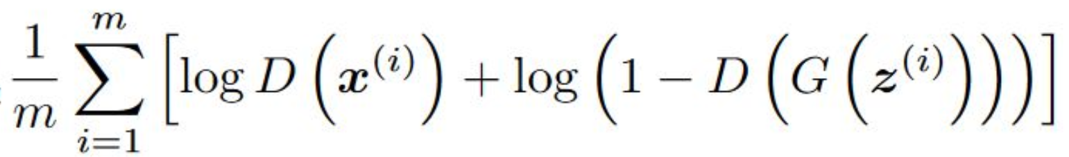
Where :

m: number of training examples.

D: Discriminator.

x(i): Training example i, so a real handwritten image.

G: Generator.

z(i): Random noise that is going to be input to the generator.

Now let's look at  a little bit more detail

• for the first term log(D(x(i))),  (x(i) is a real image) so if the discriminator can distinguish between the fake and real, it will output 1, and log(1)=0
• In the other term log(1 - D(z(i))), the generator is going to take some random noise, z(i), and it's going to output something that looks close to the real image, and the discriminator is going to output 0 if it's not fooled by the generator, and log(1-0)=0.
• At the beginning of the formula, we have just an average across all training examples m.

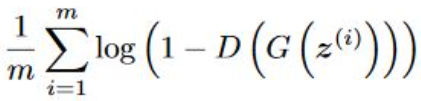
Generator loss

While the generator is trained: it samples random noise, and produces an output from that noise. The output then goes through the discriminator, and gets classified as either real or fake based on the ability of the discriminator to tell one from the other.

The generator loss is then calculated from the discriminator’s classification – it gets rewarded if it successfully fools the discriminator, and gets penalized otherwise.

The following equation is minimized to training the generator:

Putting the loss together

If we got the loss together we going to have this expression:

Where we want to minimize with respect to the generator, and we want to maximize with respect to the discriminator, this leads to this minimax game. We want to do that for some value function V that takes as input the discriminator D and the generator G, and we want to calculate the expected value of x where x comes from some real data distribution Ex~p(data(x)). We want to do that for log(D(x)). Then, we want to add the expected value of z where z comes from some random distribution Ex~p(z(z)), and we want to do that for log(1-D(G(z))).

Note:

The loss function from the generator's point of view has pretty weak gradients, so in practice, the generator is instead trained to maximize this expression as a loss function:

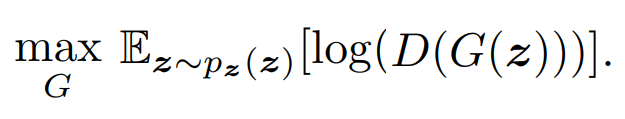
This new loss function for the generator leads to non-saturation gradients, which makes it a lot easier to training

Build our first simple GAN from scratch to generate MNIST

To learn new concepts or new software, it is better to use first a sample dataset that has no problems, and for me, the MNIST dataset is a perfect choice because it's the easiest image data to use, in our opinion. It's just like “hello world” of computer vision, and they say if something does not work in the MNIST dataset it's probably will never work.  For the upcoming tutorials, we will work with more complex data using more advanced GANs.

So in this section, we will focus to build a simple GAN from scratch to generate handwritten digits from 0 to 9.

Let's now get started with the library imports.

Load all dependencies we need

In the first step, we will import all the dependencies we need for building a simple GAN from scratch.

We first will import Numpy for linear algebra. Then, we want to use PyTorch, so let's import torch, and from torch let's import nn. That will help us in creating and training the networks (discriminator and generator), and also let's us import optim, which is a package that implements various optimization algorithms (e.g. sgd, adam,..). From torch.utils.data, let's import DataLoader to create mini batch sizes.

Note: A lot of amazing data scientists import nn and optim in this way respectevly: import torch.nn as nn, import torch.optim as optim.  

We will import also torchvision, because we are working with images obviously. From torchvision, we will import transforms and datasets to download our data and apply some transforms. Finally, we will import matplotlib.pyplot as plt to plot the results and some real samples.

import numpy as np 
import torch
from torch import nn, optim
from torch.utils.data import DataLoader
import torchvision
import torchvision.transforms as transforms
import torchvision.datasets as datasets
import matplotlib.pyplot as plt

Discriminator

Let's now build the discriminator, and from the example that I showed previously, this is going to act as our judge, so the discriminator is going to judge the image and say if it's a real or fake image.

The discriminator class will inherit from nn.Module, and it will be a very simple model that will take as input in_features which will be from the MNIST dataset, so it will be equal to 28*28*1= 784, and we will use the following layers to build our model  :

• nn.Linear: This is basically a fully connected layer
• nn.LeakyReLU: This is the activation applied to various outputs in the network, you can use nn.ReLU, but in GANs LeakyReLU is often times a better choice or better default at least.
• nn.Sigmoid(): Use it in the last layer to ensure that the result is between 0 and 1

class Discriminator(nn.Module):
    def __init__(self, in_features):
        super().__init__()
        self.disc = nn.Sequential(
            nn.Linear(in_features, 256),
            nn.LeakyReLU(0.1),
            nn.Linear(256, 128),
            nn.LeakyReLU(0.1),
            nn.Linear(128, 1),
            nn.Sigmoid()
        )
    def forward(self, x):
        return self.disc(x)

Generator

Let's now build the generator, which will generate fake handwritten digits that look like real ones, and try to fool the discriminator.

The generator class also will inherit from nn.Module, and it will be a very simple model that will take as input the noise z_dim, and generate from it the fake image. We will use the same layers to build this model, except in the final activation function we will use nn.Tanh to make sure that the output of the pixels values are between  -1 and 1. We do this because we are going to normalize the input from the MNIST dataset to ensure that it's between -1 and 1.

class Generator(nn.Module):
    def __init__(self, z_dim, img_dim):
        super().__init__()
        self.gen = nn.Sequential(
            nn.Linear(z_dim, 256),
            nn.LeakyReLU(0.1),
            nn.Linear(256, 512),
            nn.LeakyReLU(0.1),
            nn.Linear(512, img_dim),
            nn.Tanh()
        )
    def forward(self, x):
        return self.gen(x)

Hyperparameters

GANs are incredibly sensitive to hyperparameters, especially in this simple GAN. We're sort of replicating the original GAN paper in a way. In new papers, they've come to better methods to stabilize GANs, but we're going to save that for later on in upcoming articles.

DEVICE  = 'cuda' if torch.cuda.is_available() else 'cpu'
LR      = 3e-4
Z_DIM   = 64
IMG_DIM = 28*28*1
BS      = 64
EPOCHS  = 101

Initializations and preprocessing

• Initialize the discriminator and generator and take them into the device
• Set up some fixed noise to see how the same distribution images changed across the epochs
• Initialize transforms for data augmentation (RandomHorizontalFlip) and normalize our image to be between -1 and 1
• Download the MNIST dataset and apply transforms to it
• Use DataLoader to create mini batch sizes
• Initialize the optimizer for discriminator and generator, and we will use Adam for both
• Initialize the loss by BCELoss because it follows pretty much exactly the loss of GANs that we saw previously

disc        = Discriminator(IMG_DIM).to(DEVICE)
gen         = Generator(Z_DIM, IMG_DIM).to(DEVICE) 
fixed_noice = torch.randn((BS, Z_DIM)).to(DEVICE) 
transforms  = transforms.Compose([transforms.RandomHorizontalFlip(), transforms.ToTensor(),transforms.Normalize((0.5,),(0.5,))])
dataset     = datasets.MNIST(root = 'dataset/', transform = transforms, download = True)
loader      = DataLoader(dataset, batch_size=BS, shuffle=True)
opt_disc    = optim.Adam(disc.parameters(), lr=LR)
opt_gen     = optim.Adam(gen.parameters(), lr=LR)
criterion   = nn.BCELoss()

Plot some real samples

Let's plot some real samples to see how they look.

real, y = next(iter(loader))
_, ax = plt.subplots(5,5, figsize=(10,10))
plt.suptitle('Some real samples', fontsize=19, fontweight='bold')

ind = 0 
for k in range(5):
    for kk in range(5):
        ind += 1
        ax[k][kk].imshow(real[ind][0])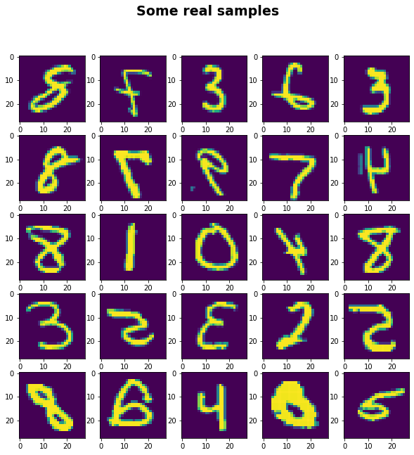

Training

Now the fun part, where the magic will happen, in this section we will train our GAN, and plot some fake samples for epochs 0, 50, and 100.

To train a GAN, we loop for all the mini batch sizes that we create with the DataLoader, and we take just the images because we don't need a label. This makes it unsupervised learning. We named the images real because they are the real ones, and we reshape them using real.view(-1, 784) to keep the number of examples in our batch, then we flatten everything else, and we take it to the device what our batch size is.

Now, let's setup the training for the discriminator. Remember, it wants to maximize log(D(real)) + log(1-D(G(z))).

To obtain the first term log(D(real)) we replace x in BCELoss by D(real) which is the output of the discriminator when it takes real images, and we replace y with ones. Our new equation will have this form:

You can notice that we are removing wn from the equation because it's just going to be one, so we can ignore it. But the important part here is that we have a minus sign in front, which means that if we want to maximize log(D(real)), then the we need to minimize the negative of that expression, and if you're used to training a neural network, you normally want to minimize the loss function.

To obtain the second term log(1-D(G(z))) we replace x in BCELoss with D(G(z)) which is the output of the discriminator when it takes fake images generated by the generator. We then replace y with zeros, so we have the following equation :

Note: To train the generator we will use also G(z), and there's no point of doing that again. When calculating the backwards loss of the discriminator, everything that was used in the forward pass to calculate those gradients have bean cleared from the cache. If we want to prevent this clearance, we add this parameter retain_graph=True.

Now let's setup the training for the generator that wants to minimize log(1-D(G(z))),  but in practice, as I said before we maximize log(D(G(z))) instead. To do so we use also BCELoss, we replace x by D(G(z)) and y by ones to obtain this equation:

Finally, we are ready to write some code to plot some fake samples, and repeat all of that as many epochs as we have.

for epoch in range(EPOCHS):
    for real,_ in loader:
        real       = real.view(-1, 784).to(DEVICE)
        batch_size = real.shape[0]
        ######## train Discriminator: max log(D(real)) + log(1-D(G(z)))
        noise     = torch.randn(batch_size, Z_DIM).to(DEVICE)
        fake      = gen(noise)
        disc_real = disc(real).view(-1) #shape [64,1] -> [64] 
        lossD_real= criterion(disc_real, torch.ones_like(disc_real))
        disc_fake = disc(fake).view(-1)
        lossD_fake= criterion(disc_fake, torch.zeros_like(disc_fake))
        lossD     = (lossD_real + lossD_fake)/2
        disc.zero_grad()
        lossD.backward(retain_graph=True) # Add retain_graph=True, To save fake in memory 
        opt_disc.step()
        
        ######## train Generator: min log(1-D(G(z))) <==> max log(D(G(z)))
        output = disc(fake).view(-1)
        lossG  = criterion(output, torch.ones_like(output))
        gen.zero_grad()
        lossG.backward()
        opt_gen.step()
        
            
    print(
                f"Epoch [{epoch}/{EPOCHS}] \
                      Loss D: {lossD:.4f}, loss G: {lossG:.4f}"
    )
    
    if epoch %50 == 0:
        with torch.no_grad():
            fake = gen(fixed_noice).reshape(-1, 1, 28, 28).cpu()
        _, ax = plt.subplots(5,5, figsize=(10,10))
        plt.suptitle('Results of epoch '+str(epoch), fontsize=19, fontweight='bold')

        ind = 0 
        for k in range(5):
            for kk in range(5):
                ind += 1
                ax[k][kk].imshow(fake[ind][0])

The images are by no means perfect, but they look alright! If you trained for longer, you can expect these to become even better. Hopefully, you will be able to follow all of the steps and get an understanding of how to implement a simple GAN for image generation.

Conclusion

In this article, we discovered why GANs are awesome by talking about some cool applications like generating realistic human faces that do not exist, restoration, colonizing, improving the resolution of photos, and transforming images across domains. Then, we broke down what GANs really are, and we gained an intuitive understanding of how they work. We dived deep into the loss function that the discriminator and generator uses, and, finally, we implemented a simple GAN from scratch to generate MNIST.

In the upcoming articles, we will explain and implement from scratch more advanced GANs to generate more cool and complex data.