Recognize these people? If not, these people call themselves The Myth Busters. Heck, they've even got a show of their own on discovery channel where they try to live up to their name, trying to bust myths like whether you can cut a jail bar by repeatedly eroding it with a dental floss. (Warning: Do not try this during your sentence).
Inspired by them, we, at Paperspace, are going do something similar. The Myth we are going to tackle is whether Batch Normalization indeed solves the problem of Internal Covariate Shift. Though Batch normalization been around for a few years and has become a staple in deep architectures, it remains one of the most misunderstood concepts in deep learning.
Does Batch Norm really solve internal covariate shift? If not, then what does it do? Is your entire deep learning education a lie? Let's find out!
Just before we begin ..
I would like to remind you that this post is a part of the series on optimization in deep learning, where we have already discussed:
- How Stochastic Gradient Descent is used to combat the problem of local minima and saddle points in deep learning.
- How adaptive methods like Momentum and Adam augment vanilla gradient descent to tackle pathological curvature in optimization surfaces.
- How different activation functions are used address the vanishing gradients problem.
One of the lessons that we took from the last post was that for neural networks to learn efficiently, the distribution that is fed to the layers of a network should be somewhat:
- Zero-centered
- Constant through time and data
The second condition means that the distribution of the data being fed to the layers should not vary too much across the mini-batches fed to the network, as well it should stay somewhat constant as the training goes on. A contrary scenario would be the distribution changing rapidly from epoch to epoch.
Internal Covariate Shift
Let's get right to the business end of things. The paper, Batch Normalization: Accelerating Deep Network Training by Reducing Internal Covariate Shift, rests on premise of addressing an issue called Internal Covariate Shift.
So, what the hey is this Internal Covariate Shift, or ICS, as we'd call it from now on. It's when the input distribution to the layers of your neural network end up fluctuating. The internal part refers to the fact that this fluctuation is happening in the intermediate layers of the neural network, which can be thought of the internal part of the network. The covariate part refers to the fact that the distributions are parameterized by weights that vary with each other. Shift, well, means the distribution is changing.
So, let's try to capture how this thing happens. Again, imagine one of the simplest neural networks possible. Linearly stacked neurons, such that you could also extend the analogy by replacing neurons with layers.

Let us suppose we are optimizing a loss function $ L $ for the network given above. The update rule of weights $ \omega_d $ of the neuron $d$ is
$$
\frac{\partial{L}}{\partial{\omega_d}} = \frac{\partial{L}}{\partial{z_d}} * \frac{\partial{z_d}}{\partial{\omega_d}}
$$
Here, $ z_d = \omega_d z_c $ is the activation of neuron $d$. Simplifying, we get,
$$
\frac{\partial{L}}{\partial{\omega_d}} = \frac{\partial{L}}{\partial{z_d}} * z_c
$$
So, we see that the gradient of the weights of the layer $d$ depends on the output of the layer $c$. The same holds true for any layer in the neural network. The gradient of the weights of a neuron depends on it's input, or the output of the layer just behind it. (Duh!)
This gradient is then backpropagated, and the weights updated. This process is repeated. Now, let us return to layer $d$.
Since we performed the gradient update for $d$, we now expect $\omega_d$ to score a lower loss. However that might not be the case. Why is that so? Let's have a closer look.
-
We perform the initial update at iteration $i$. Let us denote the distribution of output of $c$ at iteration $i$ as $ p_c^i $. Now, the update for $d$ assumes the input distribution of c as $ p_c^i $.
-
During the backward pass, however, weights of $c, \omega_c$ is also updated. This causes a shift in distribution of output of $c$.
-
In the next iteration $i+1$, suppose, the distribution of $z_c$ has shifted to $ p_c^{i + 1} $. Since the weights of the layer $d$ were updated in accordance with $ p_c^i $, and now the layer $d$ faces an input distribution $ p_c^{i+1} $, this disparity may lead to layer producing an output that doesn't decrease the loss at all.
Now, we are in a position to pose two questions.
- How exactly does a shift in distribution of the input make it harder for a layer to learn?
- Can this be shift be drastic enough to cause the scenario described above?
We answer the first question first.
Why is Internal Covariate Shift even a thing?
What neural networks do is that they generate a mapping $ f $ that maps the input $ x $ to the output $ y $. Why in the world would it make a difference if the distribution of $ x $ were to change?
I mean, look, here's when $ x $ is normally distributed.
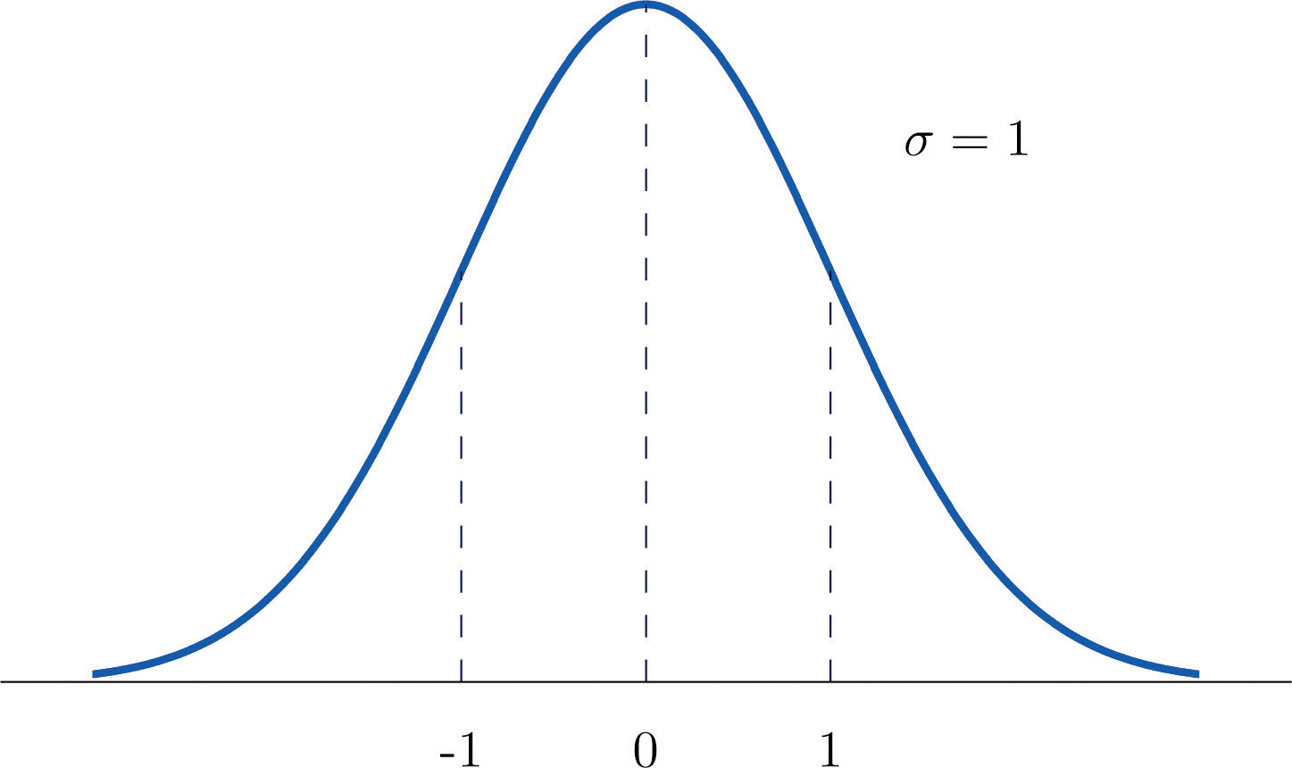
Here's when $ x $ is not normally distributed.
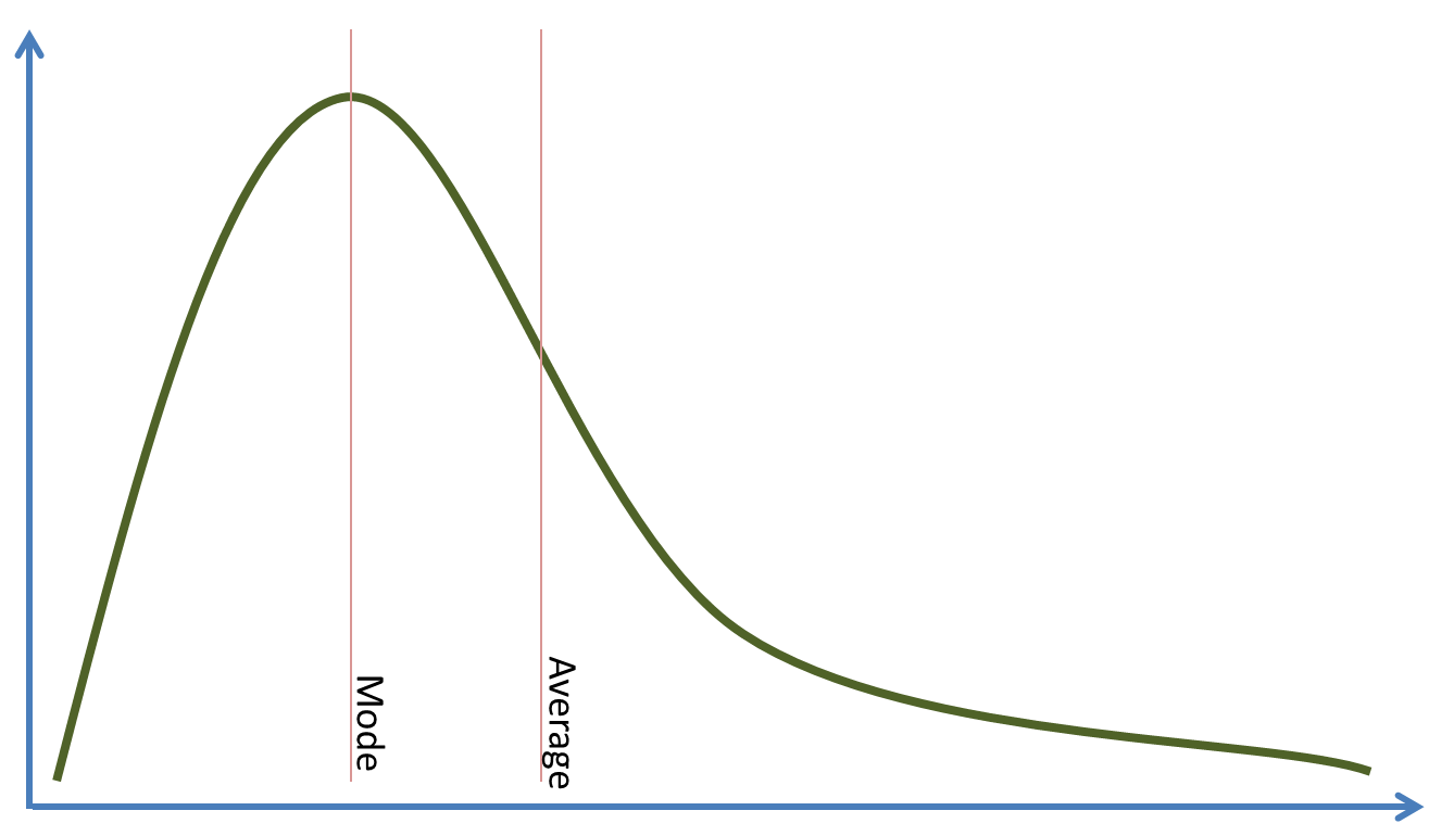
Suppose the mapping we're trying is $ f = 2x $. Why would it matter if the distribution of $ x $ has a lot of density squashed up in one place, or if it's evenly spread out.
It turns out, it does matter. It matters because neural networks, modern deep networks to be precise are insanely powerful curve-fitters. And as uncle Ben told Spiderman, "with great power comes great responsibility".
Let us suppose, we have a layer $ l $, which faces $ x $, which has a distribution given below. Also, let us suppose, the function learned by the layer $l$, up to this point in training is represented by the dashed line.

During Iteration $ i $
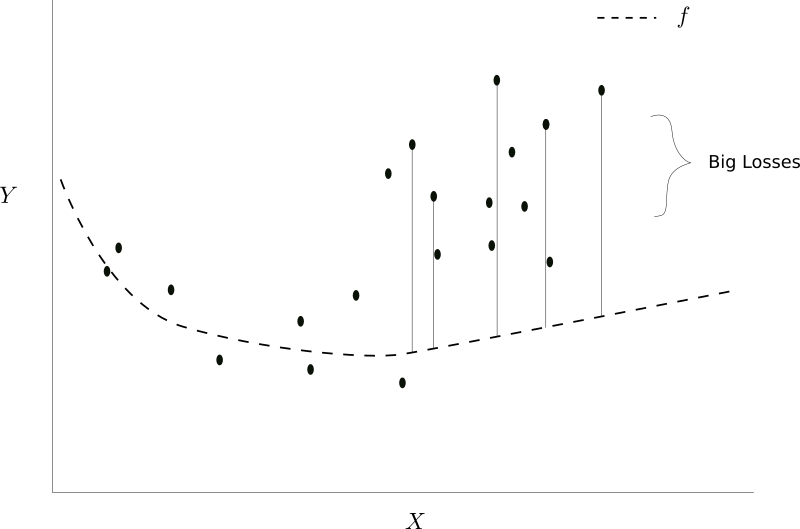
Now, suppose, after the gradient updation, the distribution of x gets changed to something like this when the next minibatch is fed to the network.
During Iteration $ i + 1 $
Notice how the loss for this mini-batch is more as compared to the previous loss. Yikes! Why does this happen?
Let's rewind to our earlier figure. You see, the mapping $f$ we learned originally does a good job of reducing the loss of the the previous mini-batch. Same is true for many other functions, which behave very differently in regions where $x$ is not dense.
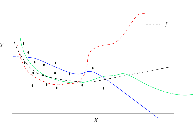
Different Functions that can fit the same input $X$ $ i $
Had we chosen the function given by the red dashed line, our loss for the next mini-batch would have been low as well.
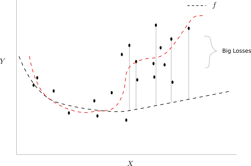
Another function would have been the better fit
But the glaring question right now is that how do we modify our algorithm so that we end up learning a mapping corresponding the red dotted line instead? The simple answer is, that there's no simple answer to this. A better to do at this point is that instead of trying to find a cure for situations like these, we rather focus our energies on preventing them in the first place.
The reason ICS ends up screwing our learning is that our neural network will always perform better on the denser regions of the input distribution. The loss for points in the denser region is reduced more as the data points in the denser region dominate the average loss, (which we are trying to minimize).
However, if ICS ends up changing the denser regions of the input distribution in subsequent batches during training, the weights learned by the network during previous iterations are no longer optimal. It will probably need a very careful tuning of the hyperparameters to get reasonable learning. This explains why ICS can be such a problem.
What we're talking is having a good amount of variance in our mini-batch. Variance makes sure that our mapping doesn't over-specialize in one region of the input distribution. We'd also like to have the mean somewhere around zero. The reason why you want to have zero-centered input to a layer has been discussed in great detail in the previous post here.
Normalizing the Inputs
One way around this problem to normalize the inputs to the neural network so that the input distribution have a zero mean and a unit variance. However, this works only when when the network is not deep enough. When the networks get deeper, say, 20 or more layers, the minor fluctuations in weights over more than 20 odd layers can produce big changes in the distribution of the input being fed to deeper layers even if the input is normalized.
One not entirely correct, but gets-the-point-across analogy is that of changes in languages. Languages change as we travel distances. However, the languages within shorter distances have a lot of similarities. Say, Spanish and Portuguese. However, both of them derive themselves from a pre-historic Indo-European language. So does Hindustani, a language spoken in India, 8,000 km away. However, the difference between Spanish and Hindustani is much larger than those between Spanish and Portuguese. The reason is that minor variations across small distances have amplified a lot. Same goes for deep networks.
Enter Batch Normalization
We now introduce the concept of Batch Normalization, which in effect, normalizes the output activations of a layer, and then does something more. Here's a precise description.
$$ \begin{gather*} y_i = BN_{\gamma,\beta}(x_i) \tag{1}\\\\ \mu_b = \frac{1}{m}\sum_{i=1}^{m}x_i \tag{2} \\\\ \sigma^2_b = \frac{1}{m}\sum_{i = 1}^m(x - \mu_b)^2 \tag{3}\\\\ \hat{x_i} = \frac{x_i - \mu_b}{\sqrt{\sigma_\beta^2 + \epsilon}} \tag{4}\\\\ \\y_i = \gamma*\hat{x_i} + \beta \tag{5} \\\\ \end{gather*} $$
The above equations describe what a batch norm layer does. Equations $2-4$ describe how mean, and variance of each activation across a mini-batch is calculated, followed by subtraction by mean to zero center the activations and dividing by the standard deviation. This is to make the standard deviation of each activation across the mini-batch unit (1).
Notice, that the mean and the variance being calculated here is the mean and the variance across the mini-batch.
The equation $5$ is where the real magic happens. $\gamma$ and $\beta$ are the hyperparameters of the so-called batch normalization layer. The output of equation $5$ has a mean of $\beta$ and a standard deviation of $\gamma$. In effect, a batch normalization layer helps our optimization algorithm to control the mean and the variance of the output of the layer.
Debunking the Myth of ICS
The paper that introduced the Batch Normalization to the world attributed it's success to the fact that it gets rid of internal covariate shift. However, that is a fallacious statement, and Batch Norm doesn't prevent ICS at all.
Internal Covariate Shift is precisely the input distribution changing as we train our network. Batch Norm has hyperparameters $\gamma$ and $\beta$ for adjusting the mean and variance of the activations. However, it does mean that as these hyperparameters are trained, they also change, and batch norm is inherently causing a changing in distribution of activations, or internal covariate shift. Had it prevented internal covariate shift, the hyperparameters $\gamma$ and $\beta$ make no sense.
So, why does Batch Norm Work?
Batch Norm doesn't cure internal covariate shift. That's for sure. If not, then why does it work at all?!
Ian Goodfellow, creator of GANs and one of the foremost researcher in field of AI has given a possible explaination in one of his lectures he delivered (The link to the lecture has been given at the end of the article). At this point, I must remind you that unless we back it up by concrete evidence, this is merely speculation, regardless the fact that it might come from one of the heavyweights in modern deep learning.
Goodfellow argues that the explaination lies at the two hyperparameters of the batch norm layer.
Let us again consider out super simple toy network.

Here. when we make a gradient update to the weights of $a$, we only compute $\frac{\partial{L}}{\partial{a}}$, that i.e. the sensitivity of the loss function with respect to $a$. However, we do not take into account that changing the weights of $a$ is also going to change the output of further layers like $b,c,d$.
Again, this really boils down to our inability to use second-order or higher-order optimization methods owing to the computational intractability of using these algorithms. Gradient Descent, along with it's variants can only capture first order interactions (We have talked about it in-depth in the part 2 of this series here).
Deep Neural networks have higher-order interactions, which means changing weights of one layer might also effect the statistics of other layers in addition to the loss function. These cross layer interactions, when unaccounted lead to internal covariate shift. Every time we update the weights of a layer, there is a chance that it effects the statistics of a layer further in the neural network in an unfavorable way.
Convergence may require careful initializing, hyperparameter tuning and longer training durations in such cases. However, when we add the batch normalized layer between the layers, the statistics of a layer are only effected by the two hyperparameters $\gamma$ and $\beta$.
Now our optimization algorithm has to adjust only two hyperparameters to control the statistics of any layer, rather than the entire weights in the previous layer. This greatly speeds up convergence, and avoids the need for careful initialization and hyperparameter tuning. Therefore, Batch Norm acts more like a check pointing mechanism.
Notice that the ability to arbitrarily set the mean and the standard deviation of a layer also means that we can recover the original distribution if that was sufficient for proper training.
Batch Norm before activation or after the activation
While the original paper talks about applying batch norm just before the activation function, it has been found in practice that applying batch norm after the activation yields better results. This seems to make sense, as if we were to put a activation after batch norm, then the batch norm layer cannot fully control the statistics of the input going into the next layer since the output of the batch norm layer has to go through an activation. This is not the case with scenario where batch norm is applied after an activation.
Batch Norm at inference
Using batch normalization during inference can be a bit tricky. This is because we might not always have a batch during inference time. For example, consider running an object detector on a video in real time. A single frame is processed at once, and hence there is no batch.
This is crucial since we need to compute the mean $\hat{x}$ and variance $\sigma^2$ of a batch to produce the output of the batch norm layer. In that case, we keep a moving average of the mean and variance during training, and then plug these values for the mean and the variance during inference. This is the approach taken by most Deep Learning libraries that ship batch norm layers out of the box.
The justification of using a moving average rests on the law of large numbers. The mean and variance of a mini-batch is a very noisy estimate of the true mean and the variance. While the batch estimates are called the batch statistics, the true (unknown to us) values of mean and variance are called the population statistics. The law of large number states, that for a large number of samples, the batch statistics will tend to converge to population statistics and that is why we use a moving average during training. It also helps us even out the noise in the estimates produced owing to the mini batch nature of our optimization algorithm.
In case, we have the option of using batches at test time, we use the same equations as above, with an exception of a minor change in the equation where we calculate the standard deviation. Instead of the equation
$$
\sigma^2_b = \frac{1}{m}\sum_{i = 1}^m(x - \mu_b)^2 \tag{3}\\
$$
we use,
$$
\sigma^2_b = \frac{1}{m-1}\sum_{i = 1}^m(x - \mu_b)^2 \tag{3}\\
$$
The reason why we use $m-1$ in the denominator instead of $m$ is that since we have already estimated the mean, we only have $m-1$ independent entities in our minibatch now. Had that not been the case, the mean could have been arbitrarily any number, but we do have a fixed mean which we are using to compute the variance. These independent entities are called degrees of freedom and a discussion on them is beyond the scope of this article.
Batch Norm as a regularizer
Batch Norm also acts a regularizer. The mean and the variance estimated for each batch is a noisier version of the true mean, and this injects randomness in our optima search. This helps in regularization.
Conclusion
While Batch Norm has been established as a standard element of deep architectures now, it's only recently that research has been directed towards understanding how it really works. A recent paper, that has been getting a lot of attention is literally titled How Does Batch Normalization Help Optimization? (No, It Is Not About Internal Covariate Shift) which demonstrates how batch norm actually ends up increasing internal covariate shift as compared to a network that doesn't use batch norm. They key insight from the paper is that batch norm actually makes the loss surface smoother, which is why it works so well. Last year, we also were introduced to SELUs or scaled Exponential Linear Unit activation functions, which implicitly normalize the activations going through them, something that is done explicitly through batch norm. The original paper for SELU contains about 100 pages of math showing how exactly that happens, and the math inclined are encouraged to read that.
Optimization is a exciting field in deep learning. While a lot of applications of deep learning have been harnessed and put to use, it's only now that we have started to scratch the enticing field of deep learning theory.
To conclude, we'd like to say.. MYTH BUSTED!


