This is the third post in the optimization series, where we are trying to give the reader a comprehensive review of optimization in deep learning. So far, we have looked at how:
-
Mini Batch Gradient Descent is used to combat local minima, and saddle points.
-
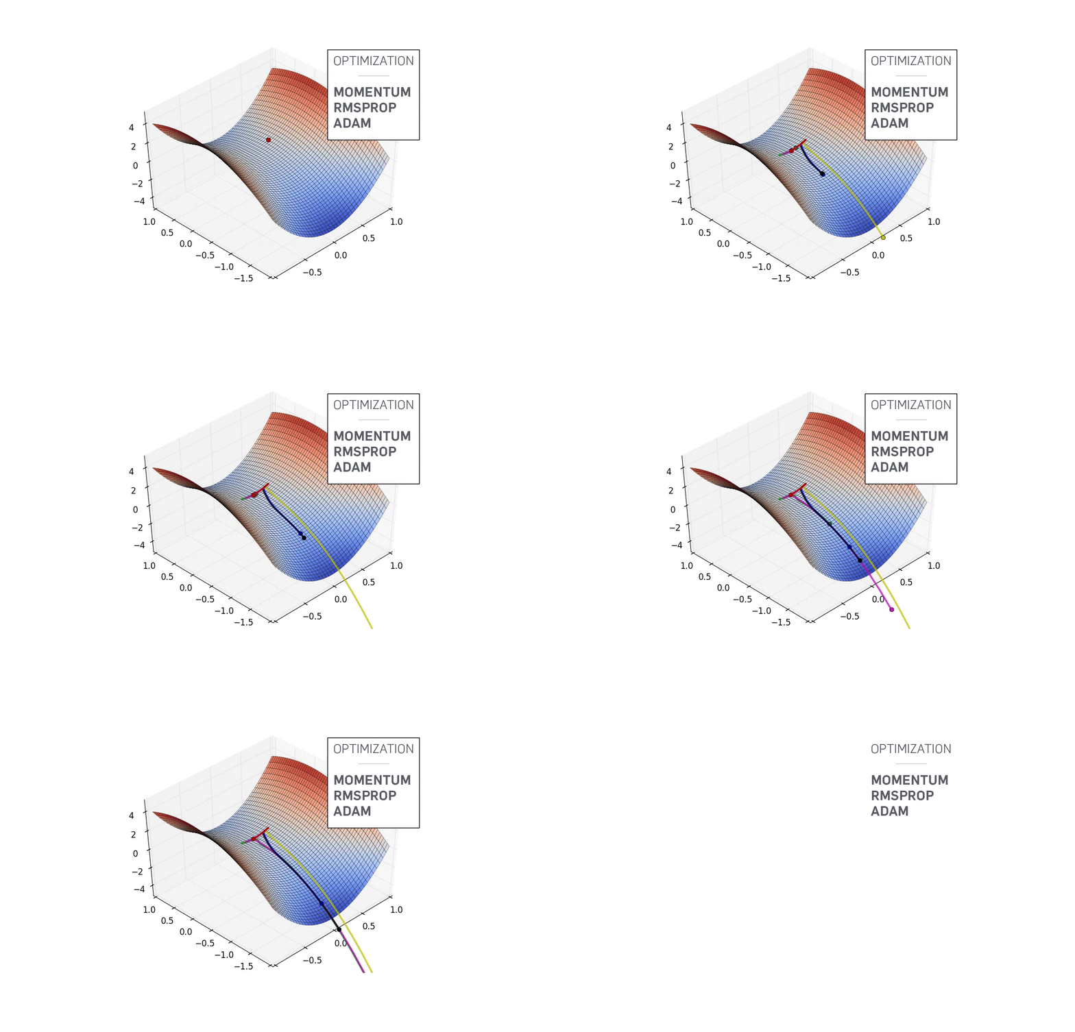
How adaptive methods like Momentum, RMSProp and Adam, augment vanilla Gradient Descent to address the problem of pathological curvature.
Distributions, Damned Distributions and Statistics
Neural networks, unlike the machine learning methods that came before it do not rest upon any probabilistic or statistical assumptions about the data they are fed. However, one of the most, if not the most important element required to ensure that neural networks learn properly is that the data fed to the layers of a neural network exhibit certain properties.
- The data distribution should be zero centered, i.e the mean of the distribution should be around zero. Absence of this can cause vanishing gradients and jittery training.
- It is preferred that the distribution be a normal one. Absence of this can cause the network to overfit to a domain of input space.
- The distributions of the activations, both across the batch as well as the across a layer, should remain somewhat constant as the training goes by. Absence of this is called Internal Covariate shift, and this may slow down training.
In this article, we will cover problems No. 1 and 2, and how activation functions are used to address them. We end with some practical advice to choose which activation function to chose for your deep network.
Vanishing Gradients
The problem of vanishing gradients is well documented, and gets much more pronounced as we go deeper and deeper with neural networks. Let us understand why they happen. Imagine the possibly simplest neural network. A bunch of neurons stacked linearly.
One can easily extend this analogy to deeper densely connected architectures. In fact, one can easily do that by replacing each neuron in the network by a full layer. Each of the neurons use a Sigmoid non-linearity as it's activation function.

The graph for a sigmoid function looks like this.
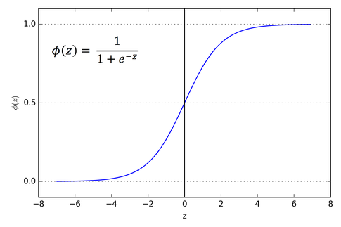
If you look at the slope of the sigmoid function, you will realize it tends to zero on either of the fringes. Or better, let us look at the plot of the gradient of the sigmoid function.
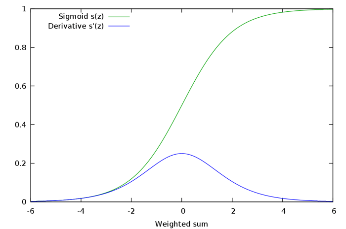
When we differentiate the output of a sigmoid activation layer with respect to it's weights , we see that the gradient of the sigmoid function is a factor in the expression. This gradient has a value ranging from 0 to 1.
$$ \frac{\partial (\sigma(\omega^Tx + b))}{\partial \omega}=\frac{\partial (\sigma(\omega^Tx + b))}{\partial (\omega^Tx + b)}*\frac{\partial (\omega^Tx + b)}{\partial \omega} $$
The second term is a sigmoid derivative, which has a range of 0 to 1.
Going back to our example, let us figure out the gradient rule for neuron A. Applying chain rule, we see that the gradient for neuron A looks like
$$ \frac{\partial L}{\partial a} = \frac{\partial L}{\partial d} * \frac{\partial d}{\partial c} * \frac{\partial c}{\partial b} * \frac{\partial b}{\partial a}
$$
Realize, that each of the term in the expression above can be further factorized to a product of gradients, one of which is a gradient of the sigmoid function. For instance,
$$ \frac{\partial d}{\partial c}=\frac{\partial d}{\partial (\sigma(\omega_d^Tc + b_d))}*\frac{\partial (\sigma(\omega_d^Tc + b_d))}{\partial (\omega_d^Tc + b_d)}*\frac{\partial (\omega_d^Tc + b_d)}{\partial c} $$
Now, let us suppose instead of 3 neurons in front of A, there are about 50 neurons in front of A. This is totally plausible in a practical scenario where networks may easily have 50 layers.
Then the gradient expression of A has a product of 50 sigmoid gradients in it, and as each such term has a value between 0 and 1, the value of the gradient of A might be driven to zero.
To see how this might happen, let's do a simple experiment. Let us randomly sample 50 numbers from 0 to 1, and then multiply them altogether.
import random
from functools import reduce

li = [random.uniform(0,1) for x in range(50)
print(reduce(lambda x,y: x*y, li))
Go try it yourself. Despite repeated attempts, I could never get a value of order more than $10^{-18}$. If this value is present in the gradient expression of neuron A as a factor, then it's gradient would be almost negligible. This means, in deeper architectures, no learning happens for the deeper neurons, or if it happens, it does so at a remarkably slower rate than the learning for the shallower higher layers.
Such a phenomenon is called the Vanishing Gradients Problem, wherein the gradients of the deeper neurons become zero or to say, vanish . The problem then is that the deeper layers of the network learn very slowly, or in worst case, the deeper layers don't learn at all.
Saturated Neurons
The problems of Vanishing gradients can be worsened by saturated neurons. Suppose, that pre-activation $\omega^Tx + b$ that is fed to a neuron with a Sigmoid activation is either very high or very low. The gradient of sigmoid at very high or low values is almost 0. Any gradient update would hardly produce a change in the weights $\omega$ and the bias $b$, and it would take a lot of steps for the neuron to get modify weights so that the pre-activation falls in an area where the gradient has a substantial value.
ReLU to the rescue
The first attempt at curbing the problem of vanishing gradients in a general deep network setting (LSTMs were introduced to combat this as well, but they were restricted to recurrent models) was the introduction of the ReLU activation function.
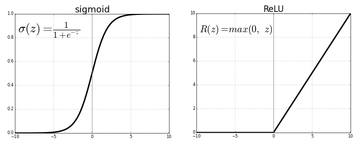
The gradient of ReLU is 1 for $x \gt 0$ and 0 for $x \lt 0$. It has multiple benefits. The product of gradients of ReLU function doesn't end up converging to 0 as the value is either 0 or 1. If the value is 1, the gradient is back propagated as it is. If it is 0, then no gradient is backpropagated from that point backwards.
One-sided Saturations
We had a two-sided saturation in the sigmoid functions. That is the activation function would saturate in both the positive and the negative direction. In contrast, ReLUs provide one-sided saturations.
Though it is not exactly precise to call the zero part of a ReLU a saturation. However, it serves the same purpose in a way that the value of the function doesn't vary at all (as opposed to very very small variation in proper saturation) as the input to the function becomes more and more negative. What benefit might a one-sided saturation bring you may ask?
We'd like to think neurons in a deep network like switches, which specialize in detecting certain features, which are often termed as concepts. While the neurons in the higher layers might end up specializing in detecting high level concepts like eyes, tyres etc, the neurons in lower layers end up specializing in low-level concepts such as curves, edges etc.
We want the neurons to fire when such a concept in present in the input it gets, and the magnitude of it is a measure of the extent of the concept in the input. For example, if a neuron detects an edge, it's magnitude might represent the sharpness of an edge.

Activation maps created by neurons learn different concepts
However, it doesn't make sense as to have an unbounded negative value for a neuron. While it's intuitive to interpret the confidence in presence of a concept, it's quite odd to to encode the absence of a concept.
Considering the example related to a neuron detecting edges, having an activation of 10 as compared as to an activation of 5 might mean a more sharper edge. But what sense does a value of -10 make when compared to -5, wherein below a value below zero represents no edge at all. Therefore, it'd be convenient to have a uniform value of zero for all the input that corresponds to the case of the concept being absent (some other concept might be present or none at all). ReLUs with their one-sided saturation accomplish exactly that.
Information Disentanglement and Robustness to Noise
Having one-sided saturation makes a neuron robust to noise. Why? Let us assume that we have a neurons values of which are unbounded, i.e. don't saturate in either of the direction. The inputs which contain the concept to varying degrees produce variance in the positive output of the neuron. This is fine as we want the magnitude to be a indicator of the strength of the signal.
However, the variance in the signal bought about background noise, or concepts the neuron doesn't specialize in (region containing arcs being fed to neurons that specialize in detecting lines) produce variance in the the negative output of the neuron .This type of variance can contribute extraneous useless information to other neurons which have dependencies with the particular neuron we are talking about. This can also lead to correlated units. For example, a neuron that detects lines might have a negative correlation with a neuron that detects arcs.
Now, let us consider the same scenario with a neuron that saturates in the negative region, (for preactivation < 0). Here, the variance due to noise, which showed up as negative magnitude earlier is squashed by the saturating element of the activation function. This prevents noise from producing extraneous signals.
Sparsity
Using a ReLu activation function also has computational benefits. ReLU based networks train quicker since no significant computation is spent in calculating the gradient of a ReLU activation. This is contrast to Sigmoid where exponentials would need to be computed in order to calculate gradients.
Since ReLU's clamp the negative preactivations to zero, they implicitly introduce sparsity in the network, which can be exploited for computational benefits.
The Dying ReLU Problem
ReLUs come with their own set of shortcomings. While sparsity is a computational advantage, too much of it can actually hamper learning. Normally, the pre-activation also contains a bias term. If this bias term becomes too negative such that $\omega^Tx + b \lt 0$, then the gradient of the ReLU activation during backward pass is 0. **Therefore, the weights and the bias causing the negative preactivations cannot be updated. **
If the weights and bias learned is such that the preactivation is negative for the entire domain of inputs, the neuron never learns, causing a sigmoid-like saturation. This is known as the dying ReLU problem.
Zero-centered activations
Since ReLUs only output non-negative activations regardless of it's input, they will always produce positive activations. This can be a drawback. Let us understand how.
For a ReLU based neural network, the gradient for any set of weights $\omega_n$ belonging to a layer $l_n$ having an activation $z_n = ReLU(\omega_n^Tx_n + b_n)$ for the loss function $L$
$$ \frac{\partial L}{\partial \omega_{n}}= \frac{\partial L}{\partial (ReLU(\omega_n^Tx_n + b_n))}*I(ReLU(\omega_n^Tx_n + b_n))*x_n $$
Here, $I(ReLU(\omega_n^Tx_n + b_n) \gt 0)$ is a indicator function which is 1 when the condition passed as it's arguement is true, and 0 otherwise. Since, a ReLU only outputs a non-negative value( $x_{n}$ ). Since each element of $x_n$ is either positive or zero, the gradient update for each weight in $\omega_n$ has the same sign as $ \frac{\partial L}{\partial (ReLU(\omega_n^Tx_n + b_n))}$
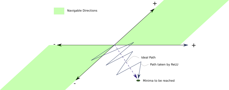
Now how is that a problem? The problem is that since the sign of gradient update for all neurons is the same, all the weights of the layer $l_n$ can either increase or decrease during one update. However, the ideal gradient weight update might be one where some weights increase while the other weights decrease. This is not possible with ReLU.
Suppose some weights need to decrease in accordance to an ideal weight update. However, if the gradient update is positive, these weights become too positive in the current iteration. In the next iteration, the gradient may be negative as well as large to remedy these increased weights, which might end up overshooting the weights which need little negative change or a positive change.
This can cause a zig zag patter in search of minima, which can slow down the training.
Problem with Leaky ReLUs
Leaky ReLUs and Parameterized ReLUs
In order to combat the problem of dying ReLUs, the leaky ReLU was proposed. A Leaky ReLU is same as normal ReLU, except that instead of being 0 for $ x \lt 0 $, it has a small negative slope for that region.
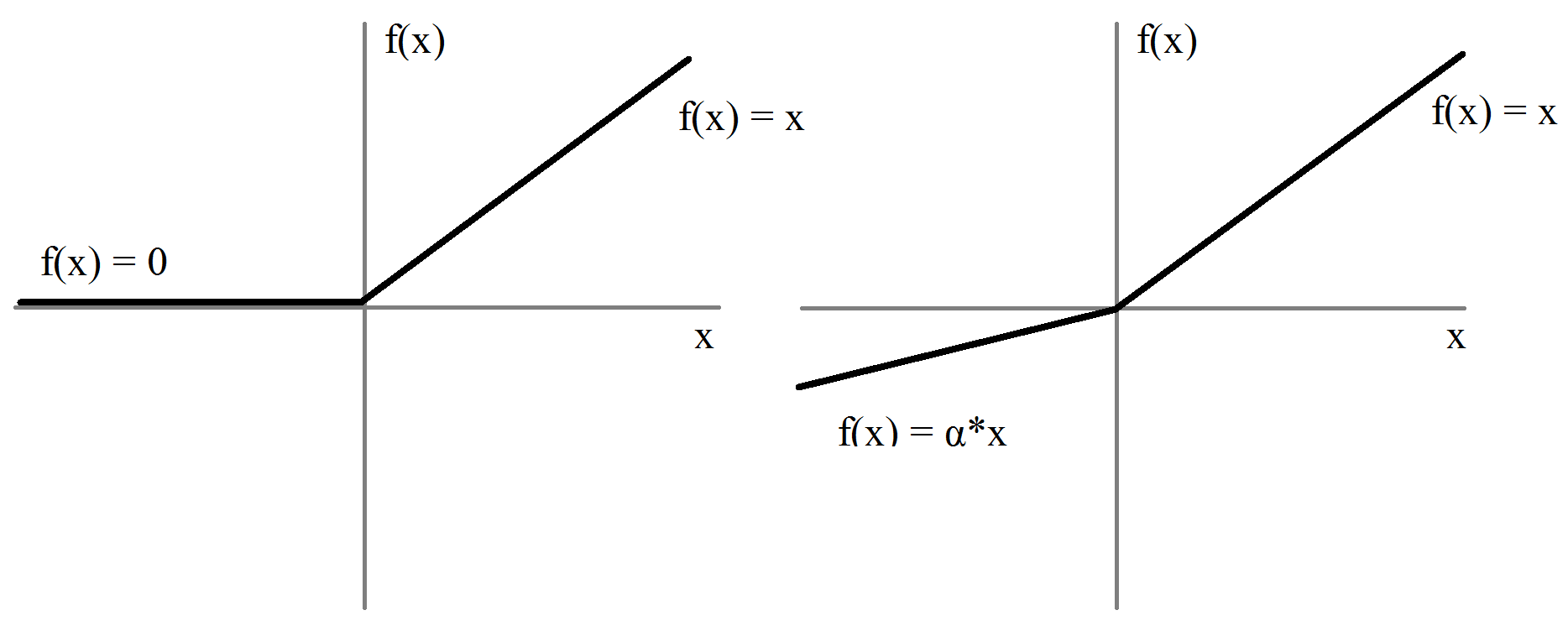
In practice, the negative slope, $\alpha$ is chosen to be a value of the order 0.01.
The benefit with Leaky ReLU's is that the backward pass is able to alter weights which produce a negative preactivation as the gradient of the activation function for inputs $ x \lt 0$ is $\alpha e^x$. For example Leaky ReLU is used in YOLO object detection algorithm.
Since, the negative pre-activations produce negative values instead of 0, we do not have the problem regarding weights being updated only in one direction that was associated with ReLU.
The value of $\alpha$ is something people have experimented quite a bit with. There exists an approach which is called Randomized Leaky ReLU, where the negative slope is randomly chosen from a uniform distribution with mean 0 and standard deviation 1.
$$ f(x)=\left\{ \begin{array}{ll} x \:\:\:\:\:\:\:\: when\:\: x \:\gt 0\\ \alpha x \:\:\:\:\:\: when \: x \leq 0\\ \end{array} \right. \\\\ \alpha \sim U(0,1) $$
The original paper of Randomized ReLU claims that it produces better and faster results than leaky ReLU and proposes, through empirical means, that if we were limited to only a single choice of $\alpha$, as in Leaky ReLU, a choice of $\frac{1}{5.5}$ would work better than 0.01
The reason why Randomized Leaky ReLU works is due to the random choice of negative slope, hence randomness of gradients for negative preactivations, which introduces randomness in the optimization algorithm. This randomness, or noise helps us steer clear of local minima and saddle points. If you need more perspective on this, I encourage you to checkout the first part of the series where we have talked in depth about the topic.
Taking the benefit of a different negative slope for each neuron, people have taken the approach further by not randomly sampling the negative slope $\alpha$ but turning it into a hyperparameter, which is learned by the network during training. Such an activation is called Parametrized ReLU.
Revisting Saturation
While neuron saturation seems like a very bad thing to have in a neural network, having one sided saturation, like we had in ReLU isn't necessarily that bad. While the above discussed variants of ReLU contribute to zero-centered activations, they don't have the benefits of one-sided saturation as discussed above.
Exponential Linear Units and Bias Shift
Following the discussion above it seems as if the perfect activation function has two desirable properties:
- Producing a zero-centered distribution, which can make the training faster.
- Having one-sided saturation which leads to better convergence.
While Leaky ReLUs and PReLU solve the first condition, they fall short on the second one. On the other hand, a vanilla ReLU satisfies the second but not the first condition.
An activation function that satisfies both the conditions is an Exponential Linear Unit (ELU).
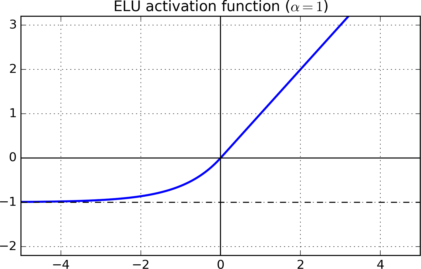
$$ f(x)=\left\{ \begin{array}{ll} x \:\:\:\:\:\:\:\:\:\:\:\:\:\:\:\:\:\:\:\:\:\:when\:\: x \:\gt 0\\ \alpha (e^{x} -1) \:\:\:\:\:\: when \: x \leq 0\\ \end{array} \right. $$
The gradient of the function is 1 for $ x \gt 0 $ while it is $ \alpha * e^x $ for $ x \lt 0 $. The function saturates for negative values to a value of $ - \alpha $. \alpha is a hyperparameter that is normally chosen to be 1.
Since, the function does have a region of negative values, we no longer have the problem of non-zero centered activations causing erratic training.
How to chose a activation function
-
Try your luck with a ReLU activation. Despite the fact we have outlined problems with ReLU, a lot of people have achieved good results with ReLU. In accordance with the principal of Occam's Razor, it's better to try out simpler stuff first. ReLUs, among all the other viable contenders have the cheapest computational budget, as well are dead simple to implement if your project requires coding up from scratch.
-
If ReLU doesn't output promising results, my next choice is a either a Leaky ReLU or a ELU. I've found that activations which are capable of producing zero centered activations are much better than the ones which don't. ELU might have been a a very easy choice, but ELU based networks are slow to train as well slow at inference time since we have to compute a lot of exponentials to compute the activation for negative preactivations. **If compute resources are not an issue for you, or if the network is not gigantic, go for ELU, other wise, you might want to stick to Leaky ReLUs. **.
Both LReLU and ELU add another hyperparameter to be tuned. -
If you have a lot of computational budget, and a lot of time, you can contrast the performance of the above activations with those of PReLU and Randomized ReLUs. Randomized ReLU can be useful if your function shows overfitting. With Parametric ReLU, you add a whole bunch of parameters to be learned to your optimisation problem. Therefore, Parameterized ReLU should be used only if you have a lot of training data.
Conclusion
In this post, we covered the need for a constant and well behaved distribution of data being fed to layers of a neural network for it learn properly. While activation functions implicitly try to normalize these distributions, a technique called Batch Normalization does this explicitly, and it wouldn't be wrong to say that it has been one of the major breakthroughs in the field of deep learning in the recent years. However, that will be covered in the next part of the series, till then, you can try your hand at trying out different activations for your network! Have fun experimenting!


