Constructing Neural Networks From Scratch: Part 2

Neural Networks are a core aspect of artificial intelligence. Almost every single concept of deep learning involves dealing with neural networks. The fundamental functionality of neural networks can be considered a black box. Most of the elements of why they work or yield the results they do are yet unknown. However, theories, hypotheses, and numerous studies help us to understand how and why these neural networks work. A deep dive into the fundamental concepts of neural networks will help us understand their functionality better.

I have covered some of the elementary concepts of how to construct neural networks from scratch in part 1 of this blog series. The viewers can check it out from the following link. We discussed some of the essential basic aspects and proceeded to build a neural network for solving different types of "Gate" Patterns. We also had a comparison and discussion on how to perform similar tasks with the deep learning frameworks. In this article, our sole focus is to cover most of the significant topics such as the implementation of layers, activation functions, and other similar concepts. The Paperspace Gradient platform is a fantastic option for the execution of the code snippets discussed in this article.

Introduction:

Constructing neural networks from scratch is one of the few methods in which an individual can master the concepts of deep learning. The knowledge of mathematics to understand the core elements of neural networks is essential. For most of the topics that we will cover in this article, we will touch on the baseline math required for understanding them. In future articles, we will cover more on the mathematic requirements, such as differentiation, which is necessary to completely understand backpropagation.

In this article, we will cover a major portion of the fundamental concepts required for the implementation of these neural networks from scratch. We will begin by constructing and implementing layers for our overall neural network architecture. Once we have the architectural layout with the layers, we will understand the core concepts of activation functions. We will then touch on the loss functions to readjust the weights and train the model appropriately to achieve the desired outcomes. Finally, we will compute all the elements we studied into a final neural network design to solve some candid tasks.

Getting started with Layers:

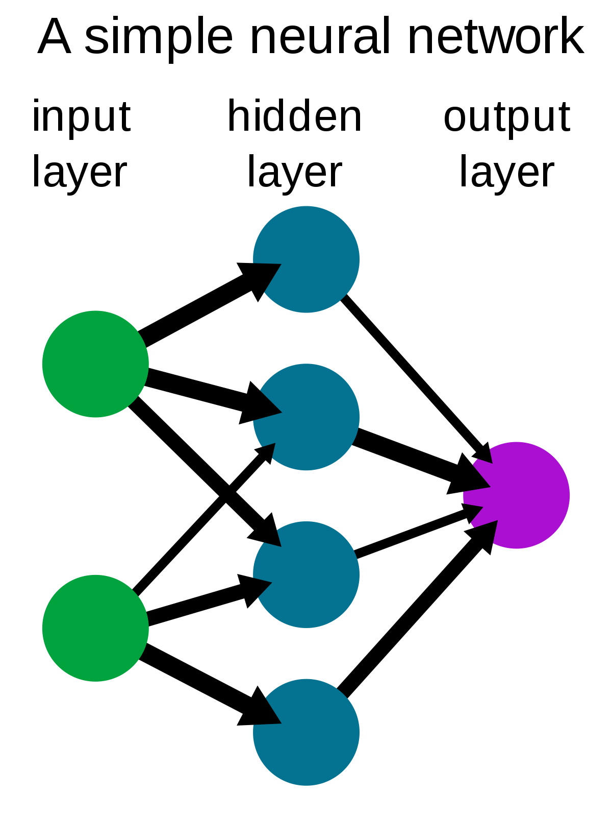
The above image shows a typical representation of a simple neural network. We have a couple of input nodes in the input layer where the data is passed through the hidden layers with four hidden nodes to finally give us a resulting output. If the viewers have thoroughly understood the first part of this article series, it is easy to correlate the AND, XOR, or other Gate problems to this neural network architecture. The input is passed through hidden layers where there is a forward propagation to the output layer.

Once the forward propagation is completed, we can compute the loss at the output layers. If the resulting value is far from the ideal solution, the resulting loss is higher. Through backpropagation, the weights of the network are readjusted to obtain a solution closer to the actual values. After training through a bunch of epochs, we can successfully train our model to learn the relative patterns accordingly. Note that in some types of problems, it is not necessary to have an input layer. The inputs can rather be passed directly through the hidden layers for further computation.

In this section, let us focus on implementing a custom "Dense" layer through which the hidden layer computations of our Neural Network can occur to perform a specific task. The hidden layers in a deep learning framework like TensorFlow or PyTorch would be their fully connected layers. The class Dense is used in the case of TensorFlow, while a Linear class is used in the case of the PyTorch library. Let us construct our own hidden Dense layer from scratch and understand how these layers work.

For building our custom layers, let us firstly import the numpy library through which we will carry out the majority of our mathematical computations. We will define a random input of the shape (3, 4) and understand how a Dense layer of a neural network works. Below is the code snippet for defining the array and printing its shape.

# Importing the numpy library and defining our input
import numpy as np

X = np.array([[0., 1., 2., 3.], 
              [3., 4., 5., 6.],
              [5., 8., 9., 7.]])

X.shape

(3, 4)

In the next step, we will define our custom class for creating the hidden (Dense) layer functionality. The first parameters initialized in the class are the number of features in each sample. This feature is always equivalent to the number of columns in your dataset. In our case, the first parameter for the number of features is four. However, the second parameter is the number of neurons that are defined by the user. The user can define how many ever the number of neurons they deem necessary for the particular task.

The random seed function is defined to get similar values per execution so that the viewers can follow along. We define random weights with the input features and the number of neurons provided by the user. We can multiply the weights with 0.1 or any other lower decimal value to ensure that the generated random numbers are less than one in the numpy array. The bias will have a shape matching the number of neurons. The forward pass function will follow the previous rules of the linear equation.

$$ Y = X * W + B $$

In the above formula, Y is the output by the neural input, X is the input, and W and B are the weights and biases, respectively. Below is the code snippet for interpreting the hidden class accordingly.

# Setting a random seed to allow better tracking
np.random.seed(42)

class Hidden:
    def __init__(self, input_features, neurons):
        # Define the random weights and biases for our statement problem
        self.weights = 0.1 * np.random.rand(input_features, neurons)
        self.bias = np.zeros((1, neurons))
        
    def forward(self, X):
        # Create the forward propagation following the formula: Y = X * W.T + B
        self.output = np.dot(X, self.weights) + self.bias

We can now proceed to create the hidden layers and perform a forward pass to receive the desired output. Below is the code snippet for performing the following action. Note that the first parameter must be four, which is the shape of the input features passed through the neural network. The second parameter, which is the number of neurons, can be anything that the user desires. The functionality is similar to the number of units passed in a Dense or Linear layer.

hidden_layer1 = Hidden(4, 10)
hidden_layer1.forward(X)
hidden_layer1.output

array([[0.30669248, 0.17604699, 0.16118867, 0.37917194, 0.3990861 ,
        0.41789485, 0.16174311, 0.18462417, 0.36694732, 0.17045874],
       [0.79104919, 0.84523964, 0.73767852, 1.01704543, 0.92694979,
        0.99778655, 0.42172713, 0.7854759 , 1.05985961, 0.61623013],
       [1.17968666, 1.4961964 , 1.34041738, 1.46314607, 1.3098747 ,
        1.49725738, 0.66537164, 1.38407469, 1.65824975, 0.93693172]])

We can also stack one hidden layer on top of the other as shown in the below code snippet.

hidden_layer2 = Hidden(10, 3)
hidden_layer2.forward(hidden_layer1.output)
hidden_layer2.output

array([[0.13752772, 0.14604601, 0.11783941],
       [0.40980827, 0.43072277, 0.37302534],
       [0.64268134, 0.67249739, 0.58861158]])

Now that we have understood some of the fundamental concepts of implementing hidden layers to our neural networks, we can proceed to understand another crucial topic of activation functions in the upcoming section of this article.

Activation Functions for Neural Networks:

When you have a set of values, and you are trying to fit a line on these values, more often than not, a single straight line cannot fit on a complex dataset as you desire. The fitting process will require some kind of external interference to adjust the model accordingly to fit on a dataset. One of the popular methods to achieve this fitting is by utilizing activation functions. As the name suggests, activating a function means activating the output nodes to vary the result in an optimal manner.

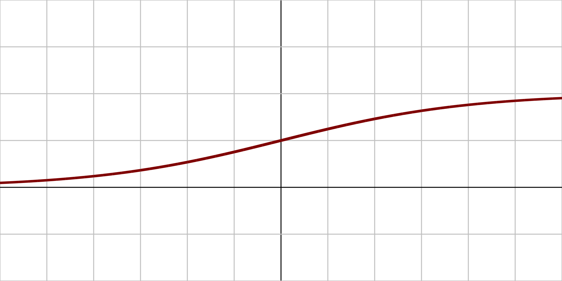
More technically, activation functions are non-linear transformations that help to activate the previous inputs before sending them over to the next output. In the late 20th century, some of the more popular options for activation functions were tanh and sigmoid. These activation functions are still utilized in the LSTM cells, and it is worth learning about them. We also used the sigmoid activation function in part 1 of this series. The working mechanisms of these activation functions are relatively simpler, but over recent years, some of their utility has been reduced.

The primary issue with these activation functions was that since their derivatives resulted in smaller values, there was often a problem of vanishing gradients. Note that the derivates are computed during the backpropagation stages to adjust the weights in the training phase. When these derivatives reach minimal values for complex tasks or larger complicated networks, it becomes futile to compute the weights as there will be no significant improvements.

One of the fixes to this solution was to use a now very popular activation function in Rectified Linear Unit (ReLU) as a replacement for these activation functions. Our primary focus on activation functions for this part of the article is the ReLU and SoftMax activation functions. Let us start by briefly analyzing and understanding each of these two essential activation functions.

ReLU Activation Function:

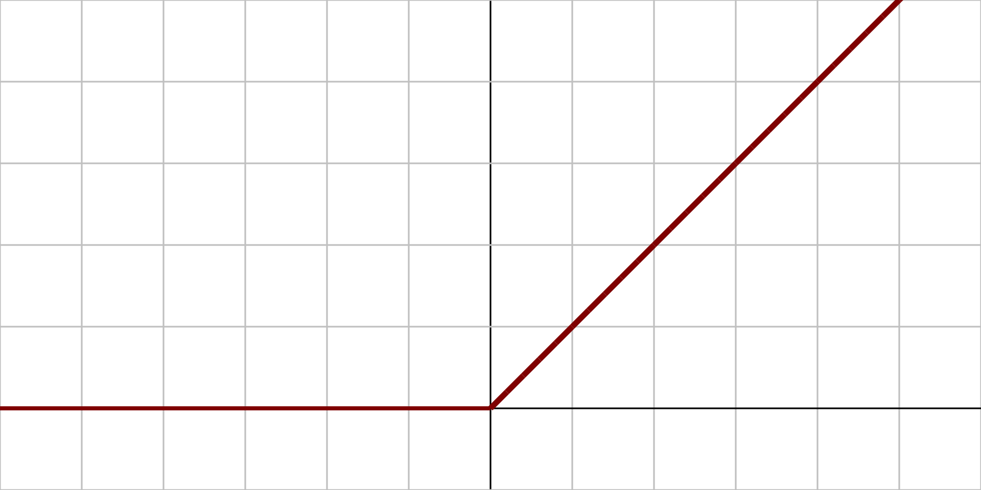
The ReLU activation function is the most popular choice among data scientists in recent times. They help to solve most of the issues that previously existed in other activation functions, such as sigmoid and tanh. As noticeable from the above graph, the ReLU function has an output of 0 when the input x values are less or equal to zero. As the value of x increases higher, the output is also activated linearly. Below is the mathematical representation of the same.

$$X =\begin{cases} 0, & if x \leq 0 \\ 1, & if x > 0 \\\end{cases}$$

The ReLU function is not continuous because it is not differentiable at the '0' point in the linear graph. This non-differentiability cause a slight issue that we will discuss later. For now, it is important to understand that the ReLU activation function returns the maximum value of the values provided that the values are greater than zero. Let us implement the ReLU activation function in our code and understand how they work in a practical example scenario. Below is the formula representation and code snippet for coding a ReLU activation function.

$$(X)^+ = max(0,  X)$$

ReLU_activation = np.maximum(0, X)

The resulting derivative values will be zero when X is less than zero and one when X is greater than one. However, the derivative output at zero is undefined. This problem can result in issues such as dying gradients, where the resulting outputs show no improvement as the weights are neutralized to none type values during backpropagation. We will need to make slight adjustments in our code to compensate for this situation or use a variation of ReLU. There are several different types of changes made to the ReLU activation function to tackle this issue accordingly. Some of these modifications include Leaky ReLU, ELU, PReLU (Parametric ReLU), and other similar variations.

SoftMax Activation Function:

In the case of Multi-class classification, activation functions like ReLU don't really work in the last layer because we have a probability distribution given by the model. In such cases, we need an activation function that is good for handling probabilities. One of the best options for multi-class classification problems is the SoftMax activation function. The SoftMax function is a combination of the exponentiation of the inputs followed by its normalization. The formulation of the SoftMax activation function can be written as follows.

$$\text{Softmax}(x_{i}) = \frac{\exp(x_i)}{\sum_j \exp(x_j)}$$

Now that we have an understanding of the formula representation of the SoftMax function, we can proceed to implement the code accordingly. We will define a random output array that we have received and try to compute the respective SoftMax loss for the same. We will compute the exponential values for each of the elements in the output array and then proceed to take the mean (or average) of these values resulting in a normalized output. This normalized output is the final result of the SoftMax function, which is basically a bunch of probabilities. We can note that the sum of these probabilities adds up to one, and the larger number has a higher probability distribution.

# Understanding Exponents and softmax basics
import numpy as np

outputs = np.array([2., 3., 4.])

# Using the above mathematical formulation to compute SoftMax
exp_values = np.exp(outputs)
mean = np.sum(exp_values)
norm_values = exp_values/mean
norm_values

array([0.09003057, 0.24472847, 0.66524096])

Note that when we perform a similar computation with a multi-dimensional array or over batches in the case of deep learning tasks, we will need to slightly modify our code accordingly. Let us import a random multi-dimensional array that we used in the previous section for further analysis. Below is the code snippet for defining the inputs.

# Importing the numpy library and defining our input
import numpy as np

X = np.array([[0., 1., 2., 3.], 
              [3., 4., 5., 6.],
              [5., 8., 9., 7.]])

The computation of the exponential values remains the same as in the last step. However, for computing the sum of the array, we will need to slightly modify our code accordingly. We are not aiming for a single value, as we need to obtain a sum for each of the input features in a particular row/batch. Hence, we will specify the axis as one to compute the elements along the row (zero for column). However, the output generated will still not match the desired array shape. We can either resize the array or set the keep dimensionality attribute as True. Below is the code snippet and the generated output.

# Computing SoftMax for an array

exp_values = np.exp(X)
mean = np.sum(exp_values, axis = 1, keepdims = True)
norm_values = exp_values / mean
norm_values

array([[0.0320586 , 0.08714432, 0.23688282, 0.64391426],
       [0.0320586 , 0.08714432, 0.23688282, 0.64391426],
       [0.01203764, 0.24178252, 0.65723302, 0.08894682]])

With that we have covered most of the intricate details required for the implementation of the SoftMax activation function. The only other issue that we might run into is the issue of explosion of values due to

Implementing Losses:

The next essential step that we will cover is the implementation of the losses for neural networks. While there are several metrics such as accuracy, F-1 Score, recall, precision, and other similar metrics, the loss function is the most useful requirement for effectively constructing neural networks. The loss function signifies the error computed during the training. The loss determines how close our predicted values are to our desired output.

There are several different types of loss functions that are used in neural networks. Out of the several different loss functions, each one of them is used for particular tasks, such as classification, segmentation, etc. Note that even though there are a few pre-defined loss functions in deep learning frameworks, you may need to define your own custom loss functions for specific tasks. We will primarily discuss two loss functions, namely mean squared error and categorical cross-entropy, for the purposes of this article.

Mean Squared Error:

The first loss function that we will briefly analyze is the mean square error. As the name suggests, we perform a mean on the square of the predicted and true values. The mean square error is one of the more straightforward approaches to calculating the loss of a neural network. At the end of the neural network at the output nodes, we compute the loss, where we compare the outcome with the expected output. In the mean squared error, we take the average of the squares of the difference between the predicted and expected values. Below is the mathematical formula and the Python code implementation of the mean square error loss.

$$ \frac{1}{n}\sum_{i=1}^{n}(y_{true} - y_{pred})^2 $$

import numpy as np

y = np.array([0., 1., 2.])
y_pred = np.array([0., 1., 1.])

mean_squared_loss = np.mean((y_pred - y) ** 2)
mean_squared_loss

0.3333333333333333

While working on projects, especially a topic like constructing neural networks from scratch, it is often a good idea to cross-verify if our implementations are computing the expected results. One of the best ways to perform such a check is to use a scientific library toolkit like scikit-learn, from which you can import the required functions for analysis. We can import the mean squared error metric available in the scikit-learn library and compute the results accordingly. Below is the code snippet for verifying your code.

# Importing the scikit-learn library for verification
from sklearn.metrics import mean_squared_error

mean_squared_error(y, y_pred)

0.3333333333333333

From the above results, it is noticeable that both the custom implementation and the verification through the scikit-learn library yield the same result. Hence, we can conclude that this implementation is correct. The readers can feel free to compute more such computations for other losses and specific metrics if required. With a brief understanding of the mean squared error, we can now proceed to further analyze the categorical cross-entropy loss function.

Categorical Cross-Entropy:

The primary loss function that we will consider for this article is categorical cross-entropy. This loss is very popular due to the success it has garnered, especially in the case of multi-class classification tasks. Typically, a categorical cross-entropy loss is followed after a final layer ending with a SoftMax activation function. For this loss, we compute the logarithmic values of the class labels linked to their respective predictions. Since the values produced by natural logarithms of values between zero and one are typically negative, we can make use of the negative (minus) sign to convert our loss function into a positive value. Below is the formula representation and the respective code snippet with the categorical cross-entropy loss output.

$$ Loss = - \sum_{i}^{} y_i \times \log{}(\hat{y_i}) $$

import numpy as np

one_hot_labels = [1, 0, 0]
preds = [0.6, 0.3, 0.1]

cat_loss = - np.log(one_hot_labels[0] * preds[0] +
                    one_hot_labels[1] * preds[1] +
                    one_hot_labels[1] * preds[1])

cat_loss

0.5108256237659907

We will cover the more intricate implementation details of the categorical cross-entropy loss in the upcoming section, where we put all the knowledge gained in this article into a single neural network. The two variations for categorical labels as well as the one-hot encoded labels will be covered while constructing the class for computing the categorical cross-entropy loss. Let us proceed to the next section to complete our architectural build.

Putting it all together to construct a neural network:

Let us combine all the knowledge we attained in this article to construct our own neural network. Firstly, we can start by importing the numpy library to perform mathematical computations and the matplotlib library for visualizing the dataset that we will work on.

# Importing the numpy library for mathematical computations and matplotlib for visualizations
import numpy as np
import matplotlib.pyplot as plt

The dataset we will utilize to test our neural network is on the neural networks case study data referred to from the following website. The spiral dataset provides the users with unique data to test their deep learning models. While data points scattered in clusters or having distinct distances between classes are easy to fit even for machine learning models, data elements that are spiral or similar in these structures tend to be harder for models to learn and adapt. Hence, if we are able to construct neural networks that are able to achieve such complex tasks, we can conclude that our networks are well built and trainable to achieve the desired task.

# Reference for the spiral dataset - https://cs231n.github.io/neural-networks-case-study/

N = 100 # number of points per class
D = 2 # dimensionality
K = 3 # number of classes
X = np.zeros((N*K,D)) # data matrix (each row = single example)
y = np.zeros(N*K, dtype='uint8') # class labels
for j in range(K):
    ix = range(N*j,N*(j+1))
    r = np.linspace(0.0,1,N) # radius
    t = np.linspace(j*4,(j+1)*4,N) + np.random.randn(N)*0.2 # theta
    X[ix] = np.c_[r*np.sin(t), r*np.cos(t)]
    y[ix] = j
    
# Visualizing the data
plt.scatter(X[:, 0], X[:, 1], c=y, s=40, cmap=plt.cm.Spectral)
plt.show()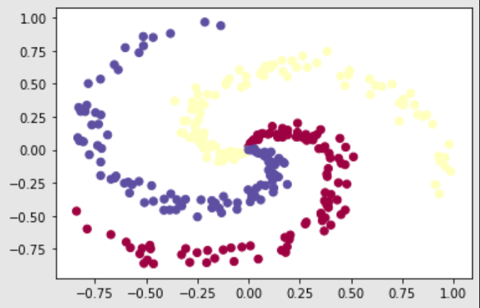

Now that we have imported the libraries and have access to the dataset, we can proceed to construct our neural network. We will first implement the hidden layer that we discussed in one of the previous sections of this article. Once we define our hidden (or dense) layers, we will also define the required activation functions that we will utilize for this task. The ReLU is the standard activation that we will use for most of the layers, while the SoftMax activation is used in the last layer for the probability distribution. Since there are three classes, we can compute our neural network accordingly with SoftMax. Note that there is a slight modification in the SoftMax code to avoid the explosion of values due to the influence of exponentiation.

The next step is to define our loss function. We will make use of the categorical cross-entropy, which is one of the more common loss functions utilized for solving multi-class classification tasks. The data is clipped on both sides. The first side is clipped to avoid division by zero, while the second side is clipped to prevent the mean from learning towards any specific value. There are two specific cases mentioned in the code snippet below. The first case is when the labels are categorical, while the second case depicts the labels are one-hot encoded. Finally, we will compute the mean of the losses for the neural network.

# Setting a random seed to allow better tracking
np.random.seed(42)

# Creating a hidden layer
class Hidden:
    def __init__(self, input_features, neurons):
        # Define the random weights and biases for our statement problem
        self.weights = 0.1 * np.random.rand(input_features, neurons)
        self.bias = np.zeros((1, neurons))
        
    def forward(self, X):
        # Create the forward propagation following the formula: Y = X * W.T + B
        self.output = np.dot(X, self.weights) + self.bias
        
# defining the ReLU activation function
class ReLU:
    def forward(self, X):
        # Compute the ReLU activation
        self.output = np.maximum(0, X)
        
# defining the Softmax activation function
class Softmax:
    # Forward pass
    def forward (self, X):
        # Get unnormalized probabilities
        exp_values = np.exp(X - np.max(X, axis = 1, keepdims = True))
        # Normalize them for each sample
        probabilities = exp_values / np.sum(exp_values, axis = 1, keepdims = True)
        self.output = probabilities
        
# Cross-entropy loss
class Loss_CategoricalCrossentropy():
    # Forward pass
    def forward (self, y_pred, y_true):
        # Number of samples in a batch
        samples = len (y_pred)
        # Clip data on both sides
        y_pred_clipped = np.clip(y_pred, 1e-7, 1 - 1e-7)
        
        # Probabilities if categorical labels
        if len (y_true.shape) == 1 :
            correct_confidences = y_pred_clipped[range (samples), y_true]
        
        # Mask values - only for one-hot encoded labels
        elif len (y_true.shape) == 2 :
            correct_confidences = np.sum(y_pred_clipped * y_true, axis = 1)
        
        # Losses
        negative_log_likelihoods = - np.log(correct_confidences)
        return negative_log_likelihoods
    
    def calculate (self, output, y):
        # Calculate sample losses
        sample_losses = self.forward(output, y)
        # Calculate mean loss
        data_loss = np.mean(sample_losses)
        # Return loss
        return data_loss

Now that we have implemented all the layers, activation functions, and losses required for our neural network, we can proceed to call the neural network elements and create the neural network architecture. We will make use of a hidden layer followed by the ReLU activation, a second hidden layer followed by the SoftMax activation, and the final categorical cross-entropy loss. Below is the code snippet and the respective result achieved.

# Defining the neural network elements
dense1 = Hidden(2, 3)
activation1 = ReLU()
dense2 = Hidden(3, 3)
activation2 = Softmax()
loss_function = Loss_CategoricalCrossentropy()

# Creating our neural network
dense1.forward(X)
activation1.forward(dense1.output)
dense2.forward(activation1.output)
activation2.forward(dense2.output)
print (activation2.output[:5])
loss = loss_function.calculate(activation2.output, y)
print ('loss:', loss)

[[0.33333333 0.33333333 0.33333333]
 [0.33332712 0.33333685 0.33333603]
 [0.33332059 0.33334097 0.33333844]
 [0.33332255 0.33332964 0.33334781]
 [0.33332454 0.33331907 0.33335639]]
loss: 1.0987351566171433

Using the knowledge we have gained throughout this article, we have been successfully able to construct our neural networks from scratch. The computed neural network model is able to have a single pass of information where the loss is computed accordingly. Even though we have touched on a lot of major aspects of neural networks in this article, we are far from covering all the essential topics. We will still need to incorporate the training process, make use of the relevant optimizers, get more familiar with differentiation, and construct more neural networks to understand their working procedure completely. My major reference for most of the aspects of this article is the Sentdex YouTube channel (and their book). I would highly recommend checking out a video guide for these concepts. We will cover the remaining information on neural networks from scratch in the next part of this series!

Conclusion:

The utility of deep learning frameworks such as TensorFlow and PyTorch can sometimes trivialize the methodology behind the construction of deep learning models. It is essential to gain a core understanding of how neural networks work to gain more conceptual and intuitive knowledge of the delicacies behind deep learning. I would once again recommend checking out the following channel for video guides to some of the sections covered in this article. Learning how to construct neural networks from scratch will allow developers to have more control and understanding over the complex deep learning tasks and projects that one must solve.

In this article, we took a look at some of the fundamental concepts required for constructing neural networks from scratch. Once we had a brief introduction to a few of the elementary topics, we proceeded to focus on the foundations of neural networks. Firstly, we understood the implementation of layers in neural networks, primarily focusing on the hidden (or dense) layers. We then touched on the significance of activation functions, namely the ReLU and SoftMax activation functions, which are extremely useful for activating the nodes to fit the model effectively. We then discussed the loss functions, namely mean squared error and categorical cross-entropy, which are useful for adjusting the weights during the training of the model. Finally, we put all the concepts together to create a neural network from scratch.

We have only covered some of the basic aspects of neural networks in the first two parts of this series. In the upcoming third part, we will look at other essential concepts such as optimizers and convolutional layers and construct more neural networks from scratch. Until then, keep programming and exploring!