Real-World Denoising Through Diffusion Model

Introduction

We can learn a great deal about our environment through images, making them an indispensable tool. However, images may be distorted by unwanted signals at any stage of the process, including capture, transmission, and storage.

The quality loss can affect image processing steps in an undesirable way. Therefore, real-world image denoising is required to clean up images before they can be used in more advanced computer vision applications without compromising the authenticity of the original data. For image identification and feature extraction to work well, real-world image denoising is required. This is because high-quality images are crucial for addressing particular challenges in a variety of fields.

(CNNs) for real-world image denoising

CNNs can self-learn features without being fed any training data or requiring any special expertise of image processing methods or statistical models. To map realistically noisy images to noise-free ones, the network can learn to account for the unique noise characteristics of the input image.

Image denoising techniques that make use of convolutional neural networks (CNNs) may be broken down into two distinct categories:

• multi-layer perceptron (MLP) models: Feedforward neural networks like MLP models can be used for  image denoising. The noisy image is fed to the input layer, and the denoised image is produced from the output layer.
• Deep learning methods: When discussing neural network topologies, the term "deep learning" is used to describe those with several hidden layers.

Here are some examples of image denoising techniques that use deep learning:

• TNRD: The trainable nonlinear reaction-diffusion model (TNRD) is a deep neural network that performs denoising by simulating the diffusion of noise in an image using a non linear, feed-forward architecture.
• FC-AIDE: FC-AIDE is a deep learning-based image denoising technique that maps noisy images to their noise-free versions using a fully convolutional neural network. This technique improves denoising performance by considering the surrounding pixels in an image. The denoising performance is also  enhanced with the use of regularization techniques.
• GCBD: Generative convolutional blind denoising (or GCBD for short). The images are "denoised" using Generative Adversarial Networks (GANs). In order to generate convincing synthetic images, GANs use a pair of neural networks called a "generator" and a "discriminator." Denoising involves training these two separate systems, one to make a noise-free version of an image(the generator) and another to detect differences between the denoised version and the original(the discriminator).

Limitations of CNN

While CNNs excel at extracting information from nearby image areas, they have trouble identifying relationships between more distant features. Some neural network architectures, like as the Transformer, employ self-attention techniques to record long-range  dependencies between data points, allowing them to function outside this restriction.

The brand-new Image Transformer was designed to be an ultra-high-resolution image generator. The Image Transformer efficiently mines global interactions between textual information using self-attention processes, residual feed-forward networks, and multi-head mechanisms.

Unlike convolutional neural networks, this design can effectively capture global data's long-range dependencies. The Image Transformer has been used to a number of image restoration tasks, such as real-world image denoising, with results that are on par with those of state-of-the-art approaches. Transformer modules are often highly large and computationally demanding, limiting their use to image restoration tasks requiring high-resolution images.

Limitations of diffusion models in real-world image denoising

• When it comes to generative modeling, diffusion models have shown to be more effective than traditional approaches. Despite their widespread use in other contexts, diffusion models have seen little adoption in the realm of practical imagine denoising. Since the final step image of standard diffusion models is characterized by Gaussian noise, regulating the amount of noise introduced in the forward process is challenging.
• The complexity and diversity of real-world noise, including its spatial and temporal dependence, frequency and color dependence, shot noise, pattern noise, and many other characteristics, has limited the use of diffusion models in real-world image denoising.

Introduction of the proposed general denoising diffusion model

The research propose a generalized real-world image denoising diffusion model using linear interpolation to solve these issues. The suggested approach uses forward gradual noise addition and backward gradual denoising operation to achieve real-world image denoising.

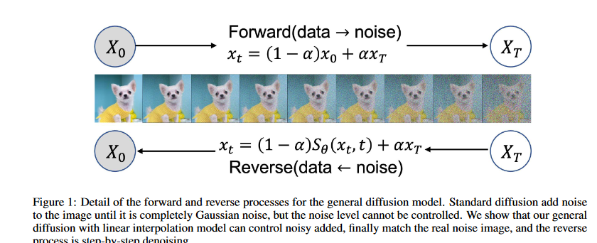
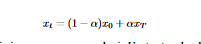
Interpolating between the original clean image and the corresponding real-world noisy image yields an intermediate noisy image. At time step t = 0, the image is the original clean image, and at time step t = T, the image corresponds to the real-world noisy image.

The amount of added noise is controlled by the parameter α = t/T, so that the noise added in the diffusion process is closer to the real world than Gaussian noise with standard distribution, thus achieving more effective image denoising.

Denoising Diffusion Probabilistic Model (DDPM)

Denoising Diffusion Probabilistic Models (DDPMs) are a type of diffusion-process-based probabilistic generative models. To simulate the distribution of images, DDPM combines a network of affine transformations with one of diffusion processes. Using the reverse diffusion algorithm as an optimization technique, the model is able to steadily enhance its generative potential through the optimization of the network's parameters.

Note: Affine transformation networks are a subset of neural networks that can be trained to perform various image transformations, including rotation, scaling, and translation. By repeatedly subjecting the image to a noise diffusion step, the diffusion process network simulates the actual diffusion process.

Diffusion process

It is possible to model the spread of particles or data over time by using a stochastic process known as a diffusion process. Diffusion models are used in the field of image processing for the purpose of denoising images by gradually diffusing the noise present in the original image. To facilitate the production of high-quality images, the DDPM model couples this diffusion process with a network that can learn the distribution of images.

DDPM has a fixed Markov chain structure for the approximate posterior q(x1:T|x0), which is also called the forward process or diffusion process . This Markov chain gradually adds Gaussian noise to the data over time, using a variance schedule β1, . . . , βT to control the amount of noise added at each point in the sequence:

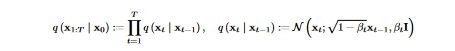
• The approximate posterior q(x1:T |x0) refers to the probability distribution of the clean image given the noisy image.
• Mean is denoted by "x sub i," where "x" is the value of the preceding pixel.
• "beta sub i" stands for the variance.
• Noise portion of the image is represented by "beta sub i" multiplied by the identity matrix "I," whereas the noise-free portion of the image is represented by the square root of "1-beta sub i" multiplied by "x sub i-1."
• For each time step, the probability distribution is a normal distribution with mean equal to the prior time step multiplied by a scaling factor of the square root of (1-beta), and variance equal to beta times the identity matrix. Here, beta is a parameter that determines how much noise is introduced to the image as a result of the diffusion operation.

Reverse diffusion

In the reverse diffusion method, a noisy image is used as a starting point, and the diffusion process is applied in reverse to clean up the image in several steps. High-quality images can be generated by the model when it has learned the underlying distribution of the clean images.

In diffusion models, the reverse process is represented by the joint distribution p (x0:T), which is specified as a Markov chain with learnt Gaussian transitions. Starting with the Gaussian distribution with mean 0 and covariance matrix I, p(xT) = N (xT ; 0, I) is the prior distribution in this chain.

Diffusion models' reverse process uses a Markov chain with learnt Gaussian transitions to smooth out noise in the image over time. The technique starts with a Gaussian distribution with mean 0 and covariance matrix I as a prior distribution, then gradually reduces the noise until the observed data is reached.

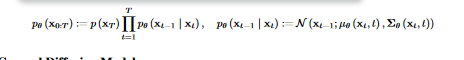
• Probability distributions for the final clean image at time T and the corresponding noisy image at time T are shown on the left, while the joint probability distribution of the intermediate noisy images at each time step from 0 to T-1 can be seen on the right.
• As the product symbol in the formula iterates itself throughout all time steps from 1 to T-1, we may infer that the generation of the intermediate noisy images is a multi-step diffusion process.
• Since linear interpolation lies at the heart of the diffusion process, the intermediate noisy image at each time step is generated by blending the original clean image with its matching real-world noisy counterpart.

General Diffusion Model

The two components of the typical diffusion model employed in image generating tasks are as follows:

• The original image undergoes a continuous random noise process that gradually adds a Gaussian distribution of noise. The noise in the image is then estimated using an Unet model trained on the original image.
• Using the same Unet model, we remove the predicted noise from a pure Gaussian image at each step to get a denoised version of the original. The final, neatly image is acquired after several iterations of this process.

In this work, the authors present  a more general diffusion model that takes into account matching the added noise to the real-world noisy image

Training algorithm for the proposed general denoising diffusion model

• The process begins by choosing two images at random from a probability distribution q. These are x0 and xT.
• A parameter known as t is used in conjunction with the formula α = t/T in order to determine the level of noise that will be introduced to the image.

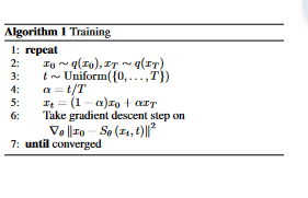
• We linearly interpolate between x0 and xT using α to generate a noisy intermediate  image, xt.
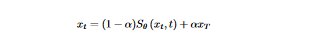
• The gradient descent is performed on the difference between the initial clean image, x0, and S(xt, t). The model's output, Sθ(xt, t), is the denoised version of xt at time t.

The proposed method results in an improved overall quality of the real-world denoised image, while allowing control of the added noise. It is essential that the output distribution xt varies continuously with respect to t, and the operator must satisfy this requirement:

The researchers employ a simple Unet network denoted Sθ to develop a sequential reverse diffusion process. This network is tailored to take in the noisy image xt and the time step t as inputs in order to estimate the target output x0. By using deep learning-driven reverse diffusion processing, the suggested network architecture allows for gradual denoising of the image.

• As we have mentionned above, xt is the intermediate noisy image at time t
• The intermediate noisy image's amount of noise can be adjusted using the parameter α;  small values of α produce a noisier image.

In practical applications, a neural network parameterized by θ must be used. The objective function of this network is to accurately restore the image x0, and this is achieved by minimizing the corresponding problem through training:

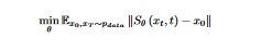
• x0 denotes a clean image randomly sampled from the distribution pdata
• xT denotes a real-world noisy image drawn from the same distribution.
• The intermediate image, denoted as xt, is obtained by interpolating between x0 and xT . In the study, the norm used is represented by ||·|| , which is specifically set to L2 within the experimental framework.

To improve performance and cope with outliers, the model is optimized using the robust Charbonnier loss rather than the standard L1 loss. The following is a definition of the Charbonnier loss:

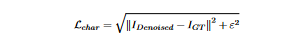
The loss function is meant to quantify the level of difference between the denoised image and the original ground truth. Denoising model performance increases as L_char decreases.

Sampling Algorithm

• The usual approach to generating an image using the diffusion model requires step-by-step sampling, and the performance of real-world image denoising is strongly reliant on the sampling technique adopted by the diffusion model.
• This research provides a step-wise sampling approach for image denoising. In the forward step, an Unet is trained to estimate x0 for images with varying degrees of noise by interpolating between clean and realistically noisy images. In the reverse process, the real-world noisy image is denoised at each stage using Sθ.

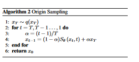
• This method is called Origin Sampling because it does an interpolation towards the original image from a sampled image. In this research, the authors evaluate this technique against another sampling algorithm which incorporates numerous enhancements to Origin Sampling to boost its performance.
• For practical image de-noising purposes, Unet performs better when S (xt, t) is equivalent to x0. This is because the accuracy of the iterative results improves across all stages of t as S gets closer to x0. Thus, real-world image denoising performance improves with a more precise assessment of x0.
• However, the accuracy of Unet is typically not very good, and errors begin to accumulate, leading to the departure of the iteration results from x0, which ultimately leads in poor image denoising performance.
• Due to the constraints imposed by the network architecture and the data sizes, the Unet is unable to make correct predictions about x0. This, in turn, causes errors to accumulate and results in erroneous iterative denoising effects. The following algorithm for carrying out denoising sampling is presented as a solution to this issue and it works better than the conventional sampling methods.

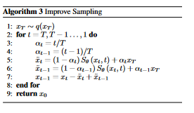
This algorithm is improved upon by the mathematical features of this sampling technique, which further improve the denoising result. For the practical image denoising task, a positive outcome may be achieved even if Sθ does not provide an

The authors of the paper "Real-World Denoising Through Diffusion Model" suggest a generic denoising diffusion model. The research provides experimental data that demonstrate that the proposed model can successfully denoise noisy images. In the paper, multiple steps were carried out:

• To train the proposed model, the authors turned to the Denoising Diffusion Implicit Models (DDIM) framework.
• The model's performance in practical denoising tasks was assessed using the CIFAR-10 dataset.
• They looked at how well the proposed model performed in comparison to BM3D, DnCNN, and NLRN, all of which are considered to be state-of-the-art denoising techniques.
• They evaluated the performance of the models using the peak signal-to-noise ratio (PSNR) and the structural similarity index (SSIM).

The experimental findings demonstrated the proposed model's superiority over the best existing denoising techniques when applied to real-world denoising tasks.. The authors showed that the proposed model can denoise noisy images in a wide range of practical settings, such as low-light photography and medical imaging.

Conclusion

This research uses a broad diffusion model with linear interpolation to give a practical approach to denoising in practice. The suggested technique combines the benefits of the simple Unet with the diffusion model, which not only uses the local receptive field of CNNs to analyze huge images but also makes use of the generative advantage of the diffusion model. In the forward step, the approach estimates the noise in the images by interpolating them using Unet. In the reverse process, the model iteratively estimates the noise and then removes it, resulting in real image denoising.

Reference

Real-World Denoising via Diffusion Model: https://arxiv.org/abs/2305.04457