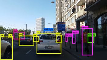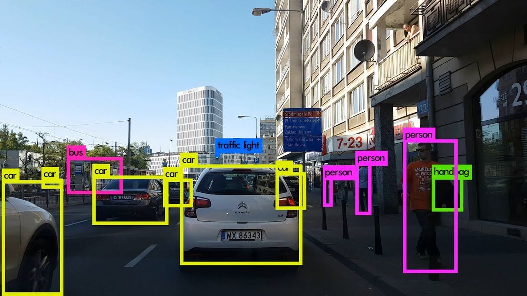
Image Credits: Karol Majek. Check out his YOLO v3 real time detection video here
This is Part 4 of the tutorial on implementing a YOLO v3 detector from scratch. In the last part, we implemented the forward pass of our network. In this part, we threshold our detections by an object confidence followed by non-maximum suppression.
The code for this tutorial is designed to run on Python 3.5, and PyTorch 0.4. It can be found in it's entirety at this Github repo.
This tutorial is broken into 5 parts:
-
Part 4 (This one): Confidence Thresholding and Non-maximum Suppression
Prerequisites
- Part 1-3 of the tutorial.
- Basic working knowledge of PyTorch, including how to create custom architectures with nn.Module, nn.Sequential and torch.nn.parameter classes.
- Basic knowledge of NumPy
In case you're lacking on any front, there are links below the post for you to follow.
In the previous parts, we have built a model which outputs several object detections given an input image. To be precise, our output is a tensor of shape B x 10647 x 85. B is the number of images in a batch, 10647 is the number of bounding boxes predicted per image, and 85 is the number of bounding box attributes.
However, as described in Part 1, we must subject our output to objectness score thresholding and Non-maximal suppression, to obtain what I will call in the rest of this post as the true detections. To do that, we will create a function called write_results in the file util.py
def write_results(prediction, confidence, num_classes, nms_conf = 0.4):
The functions takes as as input the prediction, confidence (objectness score threshold), num_classes (80, in our case) and nms_conf (the NMS IoU threshold).
Object Confidence Thresholding
Our prediction tensor contains information about B x 10647 bounding boxes. For each of the bounding box having a objectness score below a threshold, we set the values of it's every attribute (entire row representing the bounding box) to zero.
    conf_mask = (prediction[:,:,4] > confidence).float().unsqueeze(2)
    prediction = prediction*conf_mask
Performing Non-maximum Suppression
Note: I assume you understand what IoU (Intersection over union) is, and what Non-maximum suppression is. If that is not the case, refer to links at the end of the post).
The bounding box attributes we have now are described by the center coordinates, as well as the height and width of the bounding box. However, it's easier to calculate IoU of two boxes, using coordinates of a pair of diagnal corners of each box. So, we transform the (center x, center y, height, width) attributes of our boxes, to (top-left corner x, top-left corner y, right-bottom corner x, right-bottom corner y).
    box_corner = prediction.new(prediction.shape)
    box_corner[:,:,0] = (prediction[:,:,0] - prediction[:,:,2]/2)
    box_corner[:,:,1] = (prediction[:,:,1] - prediction[:,:,3]/2)
    box_corner[:,:,2] = (prediction[:,:,0] + prediction[:,:,2]/2)
    box_corner[:,:,3] = (prediction[:,:,1] + prediction[:,:,3]/2)
    prediction[:,:,:4] = box_corner[:,:,:4]
The number of true detections in every image may be different. For example, a batch of size 3 where images 1, 2 and 3 have 5, 2, 4 true detections respectively. Therefore, confidence thresholding and NMS has to be done for one image at once. This means, we cannot vectorise the operations involved, and must loop over the first dimension of prediction (containing indexes of images in a batch).
    batch_size = prediction.size(0)

    write = False

    for ind in range(batch_size):
        image_pred = prediction[ind]          #image Tensor
           #confidence threshholding
           #NMS
As describe previously, write flag is used to indicate that we haven't initialized output, a tensor we will use to collect true detections across the entire batch.
Once inside the loop, let's clean things up a bit. Notice each bounding box row has 85 attributes, out of which 80 are the class scores. At this point, we're only concerned with the class score having the maximum value. So, we remove the 80 class scores from each row, and instead add the index of the class having the maximum values, as well the class score of that class.
        max_conf, max_conf_score = torch.max(image_pred[:,5:5+ num_classes], 1)
        max_conf = max_conf.float().unsqueeze(1)
        max_conf_score = max_conf_score.float().unsqueeze(1)
        seq = (image_pred[:,:5], max_conf, max_conf_score)
        image_pred = torch.cat(seq, 1)
Remember we had set the bounding box rows having a object confidence less than the threshold to zero? Let's get rid of them.
        non_zero_ind =  (torch.nonzero(image_pred[:,4]))
        try:
            image_pred_ = image_pred[non_zero_ind.squeeze(),:].view(-1,7)
        except:
            continue

        #For PyTorch 0.4 compatibility
        #Since the above code with not raise exception for no detection
        #as scalars are supported in PyTorch 0.4
        if image_pred_.shape[0] == 0:
            continue
The try-except block is there to handle situations where we get no detections. In that case, we use continue to skip the rest of the loop body for this image.
Now, let's get the classes detected in a an image.
        #Get the various classes detected in the image
        img_classes = unique(image_pred_[:,-1]) # -1 index holds the class index
Since there can be multiple true detections of the same class, we use a function called unique to get classes present in any given image.
def unique(tensor):
    tensor_np = tensor.cpu().numpy()
    unique_np = np.unique(tensor_np)
    unique_tensor = torch.from_numpy(unique_np)

    tensor_res = tensor.new(unique_tensor.shape)
    tensor_res.copy_(unique_tensor)
    return tensor_res
Then, we perform NMS classwise.
        for cls in img_classes:
            #perform NMS
Once we are inside the loop, the first thing we do is extract the detections of a particular class (denoted by variable cls).
The following code is indented by three blocks in the original code file, but I've not indented it here because the space is limited on this page.
#get the detections with one particular class
cls_mask = image_pred_*(image_pred_[:,-1] == cls).float().unsqueeze(1)
class_mask_ind = torch.nonzero(cls_mask[:,-2]).squeeze()
image_pred_class = image_pred_[class_mask_ind].view(-1,7)

#sort the detections such that the entry with the maximum objectness
s#confidence is at the top
conf_sort_index = torch.sort(image_pred_class[:,4], descending = True )[1]
image_pred_class = image_pred_class[conf_sort_index]
idx = image_pred_class.size(0)   #Number of detections
Now, we perform NMS.
for i in range(idx):
    #Get the IOUs of all boxes that come after the one we are looking at
    #in the loop
    try:
        ious = bbox_iou(image_pred_class[i].unsqueeze(0), image_pred_class[i+1:])
    except ValueError:
        break

    except IndexError:
        break

    #Zero out all the detections that have IoU > treshhold
    iou_mask = (ious < nms_conf).float().unsqueeze(1)
    image_pred_class[i+1:] *= iou_mask

    #Remove the non-zero entries
    non_zero_ind = torch.nonzero(image_pred_class[:,4]).squeeze()
    image_pred_class = image_pred_class[non_zero_ind].view(-1,7)
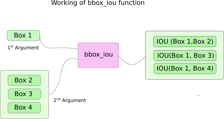
Here, we use a function bbox_iou. The first input is the bounding box row that is indexed by the the variable i in the loop.
Second input to bbox_iou is a tensor of multiple rows of bounding boxes. The output of the function bbox_iou is a tensor containing IoUs of the bounding box represented by the first input with each of the bounding boxes present in the second input.
If we have two bounding boxes of the same class having an an IoU larger than a threshold, then the one with lower class confidence is eliminated. We've already sorted out bounding boxes with the ones having higher confidences at top.
In the body of the loop, the following lines gives the IoU of box, indexed by i with all the bounding boxes having indices higher than i.
ious = bbox_iou(image_pred_class[i].unsqueeze(0), image_pred_class[i+1:])
Every iteration, if any of the bounding boxes having indices greater than i have an IoU (with box indexed by i) larger than the threshold nms_thresh, than that particular box is eliminated.
#Zero out all the detections that have IoU > treshhold
iou_mask = (ious < nms_conf).float().unsqueeze(1)
image_pred_class[i+1:] *= iou_mask

#Remove the non-zero entries
non_zero_ind = torch.nonzero(image_pred_class[:,4]).squeeze()
image_pred_class = image_pred_class[non_zero_ind]
Also notice, we have put the line of code to compute the ious in a try-catch block. This is because the loop is designed to run idx iterations (number of rows in image_pred_class). However, as we proceed with the loop, a number of bounding boxes may be removed from image_pred_class. This means, even if one value is removed from image_pred_class, we cannot have idx iterations. Hence, we might try to index a value that is out of bounds (IndexError), or the slice image_pred_class[i+1:] may return an empty tensor, assigning which triggers a ValueError. At that point, we can ascertain that NMS can remove no further bounding boxes, and we break out of the loop.
Calculating the IoU
Here is the function bbox_iou.
def bbox_iou(box1, box2):
    """
    Returns the IoU of two bounding boxes


    """
    #Get the coordinates of bounding boxes
    b1_x1, b1_y1, b1_x2, b1_y2 = box1[:,0], box1[:,1], box1[:,2], box1[:,3]
    b2_x1, b2_y1, b2_x2, b2_y2 = box2[:,0], box2[:,1], box2[:,2], box2[:,3]

    #get the corrdinates of the intersection rectangle
    inter_rect_x1 =  torch.max(b1_x1, b2_x1)
    inter_rect_y1 =  torch.max(b1_y1, b2_y1)
    inter_rect_x2 =  torch.min(b1_x2, b2_x2)
    inter_rect_y2 =  torch.min(b1_y2, b2_y2)

    #Intersection area
    inter_area = torch.clamp(inter_rect_x2 - inter_rect_x1 + 1, min=0) * torch.clamp(inter_rect_y2 - inter_rect_y1 + 1, min=0)

    #Union Area
    b1_area = (b1_x2 - b1_x1 + 1)*(b1_y2 - b1_y1 + 1)
    b2_area = (b2_x2 - b2_x1 + 1)*(b2_y2 - b2_y1 + 1)

    iou = inter_area / (b1_area + b2_area - inter_area)

    return iou
Writing the predictions
The function write_results outputs a tensor of shape D x 8. Here D is the true detections in all of images, each represented by a row. Each detections has 8 attributes, namely, index of the image in the batch to which the detection belongs to, 4 corner coordinates, objectness score, the score of class with maximum confidence, and the index of that class.
Just as before, we do not initialize our output tensor unless we have a detection to assign to it. Once it has been initialized, we concatenate subsequent detections to it. We use the write flag to indicate whether the tensor has been initialized or not. At the end of loop that iterates over classes, we add the resultant detections to the tensor output.
            batch_ind = image_pred_class.new(image_pred_class.size(0), 1).fill_(ind)
            #Repeat the batch_id for as many detections of the class cls in the image
            seq = batch_ind, image_pred_class

            if not write:
                output = torch.cat(seq,1)
                write = True
            else:
                out = torch.cat(seq,1)
                output = torch.cat((output,out))
At the end of the function, we check whether output has been initialized at all or not. If it hasn't been means there's hasn't been a single detection in any images of the batch. In that case, we return 0.
    try:
        return output
    except:
        return 0
This is it for this post. At the end of this post, we finally have a prediction in form a tensor which lists each prediction as it's row. The only thing that's left now, is to create an input pipeline to read images from disk, compute the prediction, draw bounding boxes on the images, and then display/write these images. This is what we will do in the next part.
Further Reading
Ayoosh Kathuria is currently an intern at the Defense Research and Development Organisation, India, where he is working on improving object detection in grainy videos. When he's not working, he's either sleeping or playing pink floyd on his guitar. You can connect with him on LinkedIn or look at more of what he does at GitHub