Run it on Gradient
You can follow along with the code for this tutorial and run it on a free GPU from the ML Showcase.
COVID-19 continues to wreak havoc on healthcare systems and economies around the world. With more than 500,000 dead, 11.4 million diseased, and more than a billion people put out of work, the COVID-19 pandemic is arguably the biggest crisis of the 21st century. We are also witnessing the world joining forces to fight the pandemic on an unprecedented scale–whether it be expediting trials of vaccines, mass producing masks and ventilators, or mammoth economic stimuli to keep countries going during times of lockdown.
Having said that, I am sure the Machine Learning community has a role to play. In fact, this is what this series is all about. In the last part, I gave an overview of how Deep Learning is being used to develop better ways for testing for COVID-19. All the literature that I covered used medical data procured from hospitals which was not available in the public domain, which made it hard to do any sort of tutorial. However, that has since changed.


Recently, the UC San Diego open sourced a dataset containing lung CT Scan images of COVID-19 patients, the first of its kind in the public domain. In this post we will use PyTorch to build a classifier that takes the lung CT scan of a patient and classifies it as COVID-19 positive or negative.
So, let's get started!
First thing's first...
We begin by importing the modules we will require for our code, setting up the GPU, and setting up our TensorBoard directory to log our training metrics.
import torch
import torch.nn as nn
from torch.utils.data import Dataset, DataLoader
from torchvision import transforms as transforms
from skimage.util import montage
import os
import cv2
import random
import matplotlib.pyplot as plt
import torch.optim as optim
from PIL import Image
from sklearn.metrics import classification_report, roc_auc_score, roc_curve, confusion_matrix
from torch.utils.tensorboard import SummaryWriter
import glob
import shutil
import numpy as np
from torchvision.models import vgg19_bn
import numpy as np
import seaborn as sns

random.seed(0)

log_dir = "~/logs"
writer = SummaryWriter(log_dir)
device = "cuda:0" if torch.cuda.is_available() else "cpu"
Creating the dataset
We will be using the COVID-19 CT scans provided by UC San Diego on GitHub. This dataset contains images taken from various radiology/medical journals, such as medRxiv, bioRxiv, NEJM, JAMA, Lancet.
We first start by cloning the GitHub repo to obtain the data. From the command line, run:
git clone https://github.com/UCSD-AI4H/COVID-CTOnce the data is downloaded, cd into the COVID-CT folder and extract the zip files containing the images.
cd COVID-CT/Images-processed/
unzip CT_COVID.zip
unzip CT_NonCOVID.zip

#cd back to the main folder
cd ..
About the dataset
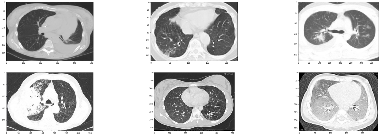
Before we start to build our classifier, let me make note of the structure of the data. We have the positive class with the scans of COVID-19 positive patients, whereas the negative class contains a mixture of healthy patients, and patients suffering from other (non-COVID-19) diseases that may cause opacities in the lungs.
In order to train a robust classifier, we must have the information about the non-COVID-19 patients as well. This is important since doctors never send a person straight to get a CT scan. In fact, since pneumonia is a clinical diagnosis, people who are put under CT Scan will probably be suffering from one of the respiratory illnesses such as viral/bacterial pneumonia/strep, etc., already. We'd seldom see a healthy patient sent for a CT scan.
Therefore, a practical classifier would have to differentiate between, say, COVID-19 induced pneumonia and other types of pneumonia. However, the negative class in this dataset is mixed up and contains healthy lungs, as well as the lungs of patients suffering from other maladies such as cancer. So what's the point of saying this? The point is that you should take this classifier as one for educational purposes. However, any classifier you want to put out in the wild would require more differentiated data.
With that in mind, let's visualize the some examples from our dataset.
Sample images from the dataset
We first begin with the COVID-19 positive cases.
covid_files_path = 'Images-processed/CT_COVID/'
covid_files      = [os.path.join(covid_files_path, x) for x in os.listdir(covid_files_path)]
covid_images    =  [cv2.imread(x) for x in random.sample(covid_files, 5)]

plt.figure(figsize=(20,10))
columns = 5
for i, image in enumerate(covid_images):
    plt.subplot(len(covid_images) / columns + 1, columns, i + 1)
    plt.imshow(image)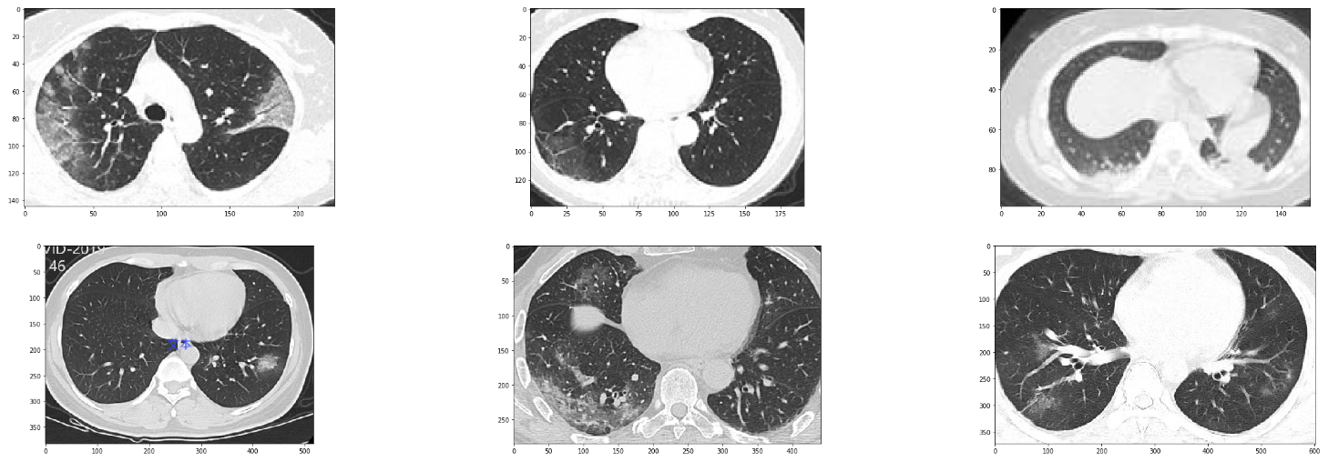
We can similarly see random samples of the non-corona cases by changing the value of covid_files_path variable to Images-processed/CT_NonCOVID.
Loading Data
The dataset is divided into three splits: the train set (425 examples), validation set (118 examples), and the test set (203 examples). Information for this split has been provided in the folder Data-split folder. This folder contains text files which explain what files belong to each split.
We write a function to read these files and put them into a list of strings.
def read_txt(txt_path):
    with open(txt_path) as f:
        lines = f.readlines()
    txt_data = [line.strip() for line in lines]
    return txt_data
We then create the COVIDCTDataset class which basically subclasses the torch.utils.data.Dataset class.
class CovidCTDataset(Dataset):
    def __init__(self, root_dir, classes, covid_files, non_covid_files, transform=None):
        self.root_dir = root_dir
        self.classes = classes
        self.files_path = [non_covid_files, covid_files]
        self.image_list = []

        # read the files from data split text files
        covid_files = read_txt(covid_files)
        non_covid_files = read_txt(non_covid_files)

        # combine the positive and negative files into a cummulative files list
        for cls_index in range(len(self.classes)):

            class_files = [[os.path.join(self.root_dir, self.classes[cls_index], x), cls_index] \
                            for x in read_txt(self.files_path[cls_index])]
            self.image_list += class_files

        self.transform = transform

    def __len__(self):
        return len(self.image_list)

    def __getitem__(self, idx):
        path = self.image_list[idx][0]

        # Read the image
        image = Image.open(path).convert('RGB')

        # Apply transforms
        if self.transform:
            image = self.transform(image)

        label = int(self.image_list[idx][1])

        data = {'img':   image,
                'label': label,
                'paths' : path}

        return data
The dataset returns a dictionary containing the image tensor, the label tensor, and a list of image paths included in the batch.
Input pre-processing and data augmentation
For the training data:
- Resize the shorter side of the image to 256 while maintaining the aspect ratio
- Do a random crop of size ranging from 50% to 100% of the dimensions of the image, and aspect ratio ranging randomly from 75% to 133% of the original aspect ratio. Finally, the crop is resized to 224 × 224
- Horizontally flip the image with a probability of 0.5
- Normalize the image to have 0 mean and standard deviation of 1
For testing:
- Resize the image to 224 × 224.
- Normalize the image to have mean 0 and standard deviation of 1
normalize = transforms.Normalize(mean=[0,0,0], std=[1,1,1])
train_transformer = transforms.Compose([
    transforms.Resize(256),
    transforms.RandomResizedCrop((224),scale=(0.5,1.0)),
    transforms.RandomHorizontalFlip(),
    transforms.ToTensor(),
    normalize
])

val_transformer = transforms.Compose([
    transforms.Resize((224,224)),
    transforms.ToTensor(),
    normalize
])
With our Dataset and DataLoader classes defined, let us now instantiate them. We use the label 0 for the non-COVID cases, whereas we use 1 for the COVID positive cases.
batchsize = 8

trainset = CovidCTDataset(root_dir='Images-processed/',
                          classes = ['CT_NonCOVID', 'CT_COVID'],
                          covid_files='Data-split/COVID/trainCT_COVID.txt',
                          non_covid_files='Data-split/NonCOVID/trainCT_NonCOVID.txt',
                          transform= train_transformer)
valset = CovidCTDataset(root_dir='Images-processed/',
                          classes = ['CT_NonCOVID', 'CT_COVID'],
                          covid_files='Data-split/COVID/valCT_COVID.txt',
                          non_covid_files = 'Data-split/NonCOVID/valCT_NonCOVID.txt',
                          transform= val_transformer)
testset = CovidCTDataset(root_dir='Images-processed/',
                          classes = ['CT_NonCOVID', 'CT_COVID'],
                          covid_files='Data-split/COVID/testCT_COVID.txt',
                          non_covid_files='Data-split/NonCOVID/testCT_NonCOVID.txt',
                          transform= val_transformer)

train_loader = DataLoader(trainset, batch_size=batchsize, drop_last=False, shuffle=True)
val_loader = DataLoader(valset, batch_size=batchsize, drop_last=False, shuffle=False)
test_loader = DataLoader(testset, batch_size=batchsize, drop_last=False, shuffle=False)
We use a mini-batch size of 8.
Performance Metrics
As we covered in Part 1, accuracy may not be enough to ascertain the efficacy of the classifier. Therefore, we need to compute metrics such sensitivity, specificity, area under ROC etc. We write the function compute_metrics to compute these metrics and some other quantities that will be useful for analysis later.
def compute_metrics(model, test_loader, plot_roc_curve = False):

    model.eval()

    val_loss = 0
    val_correct = 0

    criterion = nn.CrossEntropyLoss()

    score_list   = torch.Tensor([]).to(device)
    pred_list    = torch.Tensor([]).to(device).long()
    target_list  = torch.Tensor([]).to(device).long()
    path_list    = []


    for iter_num, data in enumerate(test_loader):

        # Convert image data into single channel data
        image, target = data['img'].to(device), data['label'].to(device)
        paths = data['paths']
        path_list.extend(paths)

        # Compute the loss
        with torch.no_grad():
            output = model(image)

        # Log loss
        val_loss += criterion(output, target.long()).item()


        # Calculate the number of correctly classified examples
        pred = output.argmax(dim=1, keepdim=True)
        val_correct += pred.eq(target.long().view_as(pred)).sum().item()

        # Bookkeeping
        score_list   = torch.cat([score_list, nn.Softmax(dim = 1)(output)[:,1].squeeze()])
        pred_list    = torch.cat([pred_list, pred.squeeze()])
        target_list  = torch.cat([target_list, target.squeeze()])


    classification_metrics = classification_report(target_list.tolist(), pred_list.tolist(),
                                                  target_names = ['CT_NonCOVID', 'CT_COVID'],
                                                  output_dict= True)


    # sensitivity is the recall of the positive class
    sensitivity = classification_metrics['CT_COVID']['recall']

    # specificity is the recall of the negative class
    specificity = classification_metrics['CT_NonCOVID']['recall']

    # accuracy
    accuracy = classification_metrics['accuracy']

    # confusion matrix
    conf_matrix = confusion_matrix(target_list.tolist(), pred_list.tolist())

    # roc score
    roc_score = roc_auc_score(target_list.tolist(), score_list.tolist())

    # plot the roc curve
    if plot_roc_curve:
        fpr, tpr, _ = roc_curve(target_list.tolist(), score_list.tolist())
        plt.plot(fpr, tpr, label = "Area under ROC = {:.4f}".format(roc_score))
        plt.legend(loc = 'best')
        plt.xlabel('False Positive Rate')
        plt.ylabel('True Positive Rate')
        plt.show()


    # put together values
    metrics_dict = {"Accuracy": accuracy,
                    "Sensitivity": sensitivity,
                    "Specificity": specificity,
                    "Roc_score"  : roc_score,
                    "Confusion Matrix": conf_matrix,
                    "Validation Loss": val_loss / len(test_loader),
                    "score_list":  score_list.tolist(),
                    "pred_list": pred_list.tolist(),
                    "target_list": target_list.tolist(),
                    "paths": path_list}


    return metrics_dict
Define the Model
We now define our model. We use the pretrained VGG-19 with batch normalization as our model. We then replace its final linear layer with one having 2 neurons at its output, and perform transfer learning over our dataset.
We use cross entropy loss as our objective function.
model = vgg19_bn(pretrained=True)
model.classifier[6] = nn.Linear(4096, 2)
model.to(device)
Now, you can also try other models such as ResNet, DenseNet etc., especially if you are looking for lighter models, since VGG-19 has more parameters than either ResNet or DenseNet. My choice for going for VGG is that it often leads to more intuitive activation maps.
In case you want to use another model, make sure you replace the final layer to have two outputs.
Training Hyperparameters
We now set the training hyperparameters. We use an initial learning rate of 0.01. We used Stochastic Gradient descent with momentum value of 0.9.
learning_rate = 0.01
optimizer     = optim.SGD(model.parameters(), lr = learning_rate, momentum=0.9)
Early Stopping
We implement a class called EarlyStopping which keeps the running averages of both loss and accuracy. This will help us in implementing, well, you guessed it–early stopping.
This class keeps a moving average of the loss and accuracy. If the metric doesn't improve beyond a set number of epochs, defined by the patience, then the method stop returns:
0, if patience has not been exhausted for either accuracy or the loss
1, if patience is exhausted for both the accuracy and the loss
2, if patience has been exhausted only for accuracy
3, if patience has been exhausted only for loss
Note that the usage of the term patience has been exhausted for a metric means that the metric has not been improving for a set number of epochs.
from collections import deque

class EarlyStopping(object):
    def __init__(self, patience = 8):
        super(EarlyStopping, self).__init__()
        self.patience = patience
        self.previous_loss = int(1e8)
        self.previous_accuracy = 0
        self.init = False
        self.accuracy_decrease_iters = 0
        self.loss_increase_iters = 0
        self.best_running_accuracy = 0
        self.best_running_loss = int(1e7)

    def add_data(self, model, loss, accuracy):

        # compute moving average
        if not self.init:
            running_loss = loss
            running_accuracy = accuracy
            self.init = True

        else:
            running_loss = 0.2 * loss + 0.8 * self.previous_loss
            running_accuracy = 0.2 * accuracy + 0.8 * self.previous_accuracy

        # check if running accuracy has improved beyond the best running accuracy recorded so far
        if running_accuracy < self.best_running_accuracy:
            self.accuracy_decrease_iters += 1
        else:
            self.best_running_accuracy = running_accuracy
            self.accuracy_decrease_iters = 0

        # check if the running loss has decreased from the best running loss recorded so far
        if running_loss > self.best_running_loss:
            self.loss_increase_iters += 1
        else:
            self.best_running_loss = running_loss
            self.loss_increase_iters = 0

        # log the current accuracy and loss
        self.previous_accuracy = running_accuracy
        self.previous_loss = running_loss


    def stop(self):

        # compute thresholds
        accuracy_threshold = self.accuracy_decrease_iters > self.patience
        loss_threshold = self.loss_increase_iters > self.patience


        # return codes corresponding to exhuaustion of patience for either accuracy or loss
        # or both of them
        if accuracy_threshold and loss_threshold:
            return 1

        if accuracy_threshold:
            return 2

        if loss_threshold:
            return 3


        return 0

    def reset(self):
        # reset
        self.accuracy_decrease_iters = 0
        self.loss_increase_iters = 0

early_stopper = EarlyStopping(patience = 5)
Training Loop
If the patience for running validation loss is exhausted, but not for running accuracy, we multiply our learning rate by 0.1. If patience for both running validation loss and running accuracy is exhausted, we stop the training.
The reasons for such a policy lies in the nature of the cross entropy loss, where a higher validation loss may not necessarily correspond to a lower accuracy. Why? Because one of the subtleties of Cross Entropy loss is that it prefers high confidence predictions. So a more accurate model which is less confident about its predictions may have a higher loss than the model with lower accuracy but very confident predictions. Therefore, we make the decision only to stop when the accuracy stops increasing as well.
We train for a maximum of 60 epochs.
A note on batch size
As you saw, I used a batch size of 8. However, to get good results you must use a higher batch size, say 64 or 128. My RTX 2060 could only fit a batch size of 8. To essentially achieve a batch update of size 64, we can accumulate the gradient over 8 iterations ( 8 (batch size) * 8 (iterations) = 64) and perform a gradient update only then. The basic template for doing this is very straight forward.
loss += one_iter_loss / 8
if i %% 8 == 0:
	loss.backward()
We divide the loss by 8 since we are adding updates for 8 iterations, and we need to rescale the loss.
Here is the code for the training loop. It's a big chunk of code, so I have put in comments so that you can easily follow along.
best_model = model
best_val_score = 0

criterion = nn.CrossEntropyLoss()

for epoch in range(60):

    model.train()
    train_loss = 0
    train_correct = 0

    for iter_num, data in enumerate(train_loader):
        image, target = data['img'].to(device), data['label'].to(device)

        # Compute the loss
        output = model(image)
        loss = criterion(output, target.long()) / 8

        # Log loss
        train_loss += loss.item()
        loss.backward()

        # Perform gradient udpate
        if iter_num % 8 == 0:
            optimizer.step()
            optimizer.zero_grad()


        # Calculate the number of correctly classified examples
        pred = output.argmax(dim=1, keepdim=True)
        train_correct += pred.eq(target.long().view_as(pred)).sum().item()


    # Compute and print the performance metrics
    metrics_dict = compute_metrics(model, val_loader)
    print('------------------ Epoch {} Iteration {}--------------------------------------'.format(epoch,
                                                                                                 iter_num))
    print("Accuracy \t {:.3f}".format(metrics_dict['Accuracy']))
    print("Sensitivity \t {:.3f}".format(metrics_dict['Sensitivity']))
    print("Specificity \t {:.3f}".format(metrics_dict['Specificity']))
    print("Area Under ROC \t {:.3f}".format(metrics_dict['Roc_score']))
    print("Val Loss \t {}".format(metrics_dict["Validation Loss"]))
    print("------------------------------------------------------------------------------")

    # Save the model with best validation accuracy
    if metrics_dict['Accuracy'] > best_val_score:
        torch.save(model, "best_model.pkl")
        best_val_score = metrics_dict['Accuracy']


    # print the metrics for training data for the epoch
    print('\nTraining Performance Epoch {}: Average loss: {:.4f}, Accuracy: {}/{} ({:.0f}%)\n'.format(
        epoch, train_loss/len(train_loader.dataset), train_correct, len(train_loader.dataset),
        100.0 * train_correct / len(train_loader.dataset)))

    # log the accuracy and losses in tensorboard
    writer.add_scalars( "Losses", {'Train loss': train_loss / len(train_loader), 'Validation_loss': metrics_dict["Validation Loss"]},
                                   epoch)
    writer.add_scalars( "Accuracies", {"Train Accuracy": 100.0 * train_correct / len(train_loader.dataset),
                                       "Valid Accuracy": 100.0 * metrics_dict["Accuracy"]}, epoch)

    # Add data to the EarlyStopper object
    early_stopper.add_data(model, metrics_dict['Validation Loss'], metrics_dict['Accuracy'])

    # If both accuracy and loss are not improving, stop the training
    if early_stopper.stop() == 1:
        break

    # if only loss is not improving, lower the learning rate
    if early_stopper.stop() == 3:
        for param_group in optimizer.param_groups:
            learning_rate *= 0.1
            param_group['lr'] = learning_rate
            print('Updating the learning rate to {}'.format(learning_rate))
            early_stopper.reset()
As this network trains, you can see the the training/validation accuracy and losses being plotted in TensorBoard by going to the directory logs and running TensorBoard from it.
cd logs
tensorboard --logdir .
Testing Performace
For testing, you could use either of these options:
- Latest model
- Load the model with the best validation accuracy which is stored as
best_model.pkl. To load it, usemodel = torch.load('best_model.pkl) - Pre-trained model provided here. Download the model and use
model = torch.load('pretrained_covid_model.pkl'). Download the pretrained model from here.
Once you have loaded the model, you can compute the performance metrics using the following code.
model = torch.load("pretrained_covid_model.pkl" )

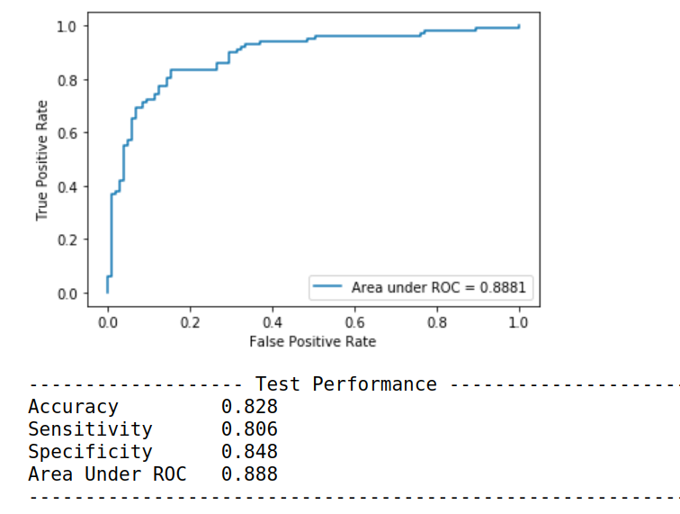
metrics_dict = compute_metrics(model, test_loader, plot_roc_curve = True)
print('------------------- Test Performance --------------------------------------')
print("Accuracy \t {:.3f}".format(metrics_dict['Accuracy']))
print("Sensitivity \t {:.3f}".format(metrics_dict['Sensitivity']))
print("Specificity \t {:.3f}".format(metrics_dict['Specificity']))
print("Area Under ROC \t {:.3f}".format(metrics_dict['Roc_score']))
print("------------------------------------------------------------------------------")
Running this piece of code produces:
You can also print the confusion matrix of the model.
conf_matrix = metrics_dict["Confusion Matrix"]
ax= plt.subplot()
sns.heatmap(conf_matrix, annot=True, ax = ax, cmap = 'Blues'); #annot=True to annotate cells

# labels, title and ticks
ax.set_xlabel('Predicted labels');ax.set_ylabel('True labels');
ax.set_title('Confusion Matrix');
ax.xaxis.set_ticklabels(['CoViD', 'NonCoViD']); ax.yaxis.set_ticklabels(['CoViD', 'NonCoViD']);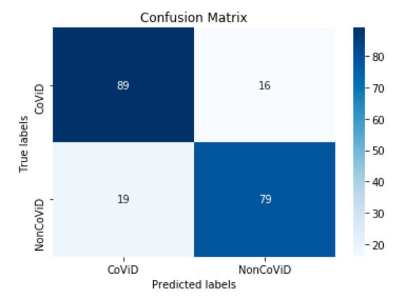
Identifying Mistakes
We now look at the the mistakes that our model has committed. We first get the indices of the misclassified examples. Then we look at the scores assigned to the misclassified examples and plot a histogram.
targets = np.array(metrics_dict['target_list'])
preds   = np.array(metrics_dict['pred_list'])
scores  = np.array(metrics_dict['score_list'])


misclassified_indexes = np.nonzero(targets != preds)
misclassified_scores = scores[misclassified_indexes[0]]

# plot the historgram of misclassified scores
plt.hist(misclassified_scores)
plt.xlabel("scores")
plt.ylabel("No. of examples")
plt.show()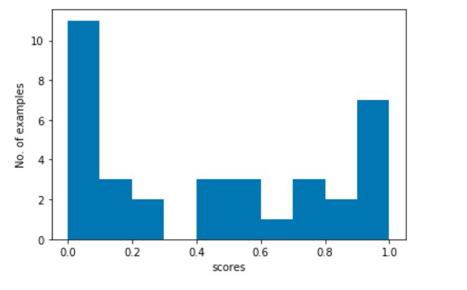
We plot the scores to see the nature of mistakes our model commits. Mistakes for examples with scores near 0.5 (our threshold) means that our model is ambiguous about these examples. We also see spikes at both ends, 0.0 and 1.0. This means that the model is very confident in misclassifying these examples.
Using Grad-CAM to visualise activations
Gradient-weighted Class Activation Mapping, or more simply Grad-CAM, helps us get what the network is seeing, and helps us see which neurons are firing in a particular layer given the image as input.
We first begin by cloning the requisite repo implementing Grad-CAM.
!git clone https://github.com/jacobgil/pytorch-grad-cam
!mv pytorch-grad-cam gradcam
Now we define a function called do_grad_cam which takes the path of an image and outputs an image with the Grad-CAM mask.
from gradcam.gradcam import *

def do_grad_cam(path):

    # Initialise the grad cam object.
    # we use model.features as the feature extractor and use the layer no. 35 for gradients.
    grad_cam = GradCam(model=model, feature_module=model.features, \
                           target_layer_names=["35"], use_cuda=True)

    # read in the image, and prepare it for the network
    orig_im = cv2.imread(path)
    img = Image.fromarray(orig_im)
    inp = val_transformer(img).unsqueeze(0)

    # main inference
    mask = grad_cam(inp, None)

    # create the heatmap
    heatmap = cv2.applyColorMap(np.uint8(255 * mask), cv2.COLORMAP_JET)
    heatmap = np.float32(heatmap) / 255

    #add the heatmap to the original image
    cam = heatmap + np.float32(cv2.resize(orig_im, (224,224))/255.)
    cam = cam / np.max(cam)

    # BGR -> RGB since OpenCV operates with BGR values.
    cam = cam[:,:,::-1]

    return cam
Let us now use the grad cam functionality to visualize a few examples from True positives, True negatives, False positives and False negatives.
True Positives
true_positives = np.logical_and(preds == 1, targets == 1)
true_positives = np.logical_and(true_positives, scores > 0.9)
true_positives_indices = np.nonzero(true_positives)
true_positives_paths = [metrics_dict['paths'][i] for i in true_positives_indices[0]]


true_positive_images    =  [do_grad_cam(x) for x in random.sample(true_positives_paths, 10)]

plt.figure(figsize=(30,15))
columns = 5
for i, image in enumerate(true_positive_images):
    plt.subplot(len(true_positive_images) / columns + 1, columns, i + 1)
    plt.imshow(image)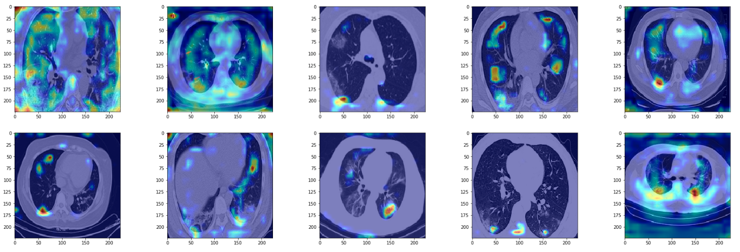
We see the model is able to focus on the ground-glass deformities that are characteristic of CT scans of COVID-infected patients. However, we also see that at times the network focuses on the boundary of the lung (in gray color) to make the decision. I am no radiologist to say whether we should be looking at the boundary to make the decision, but if not, then this is something that merits further inspection.
False Positives
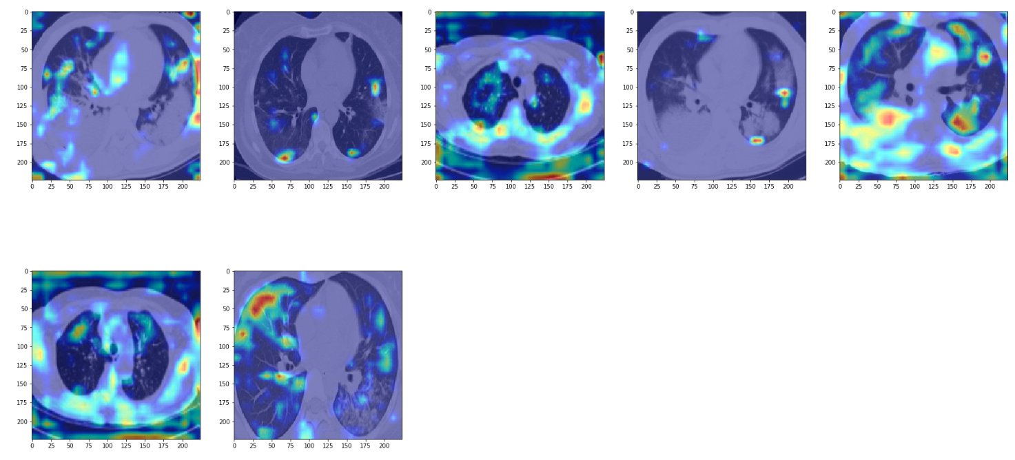
In these examples, we see that the network focuses again on opacities but it isn't quite efficient enough to identify opacities corresponding to non-COVID pneumonia from COVID pneumonia.
True Negatives
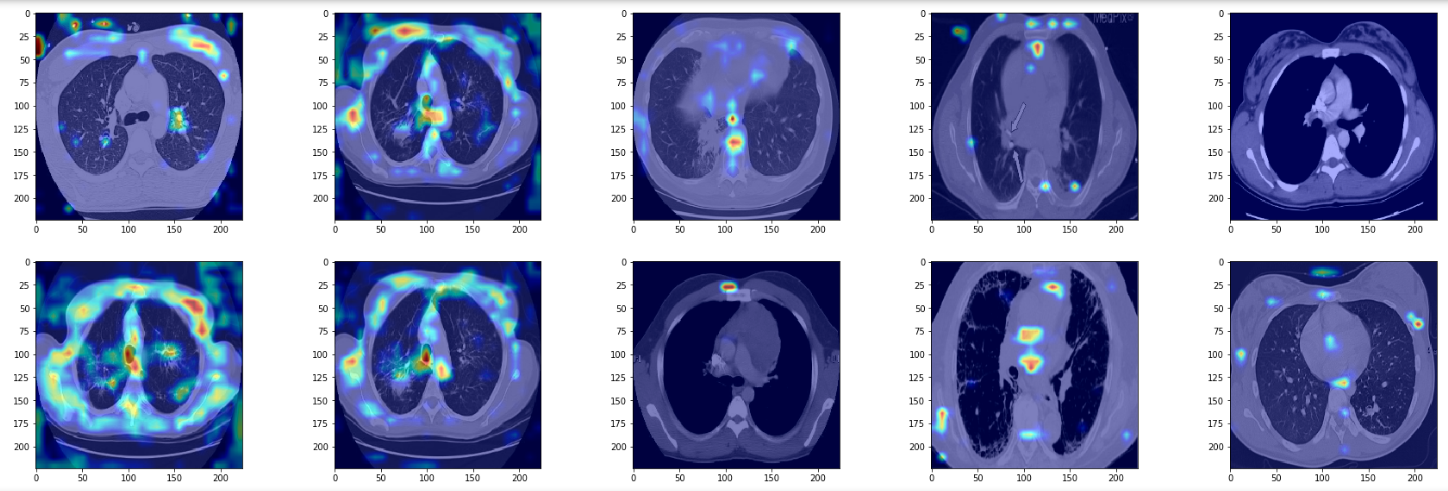
In true negatives, the network seems to be focusing more on the lung boundary rather than the opacities in the lung. The opacities it sees are not very dense, or ground-glass like. Again, since I'm no radiologist I may be totally off track, but it seems as if the model depends on scarcity of opacities to make the negative prediction.
False Negatives
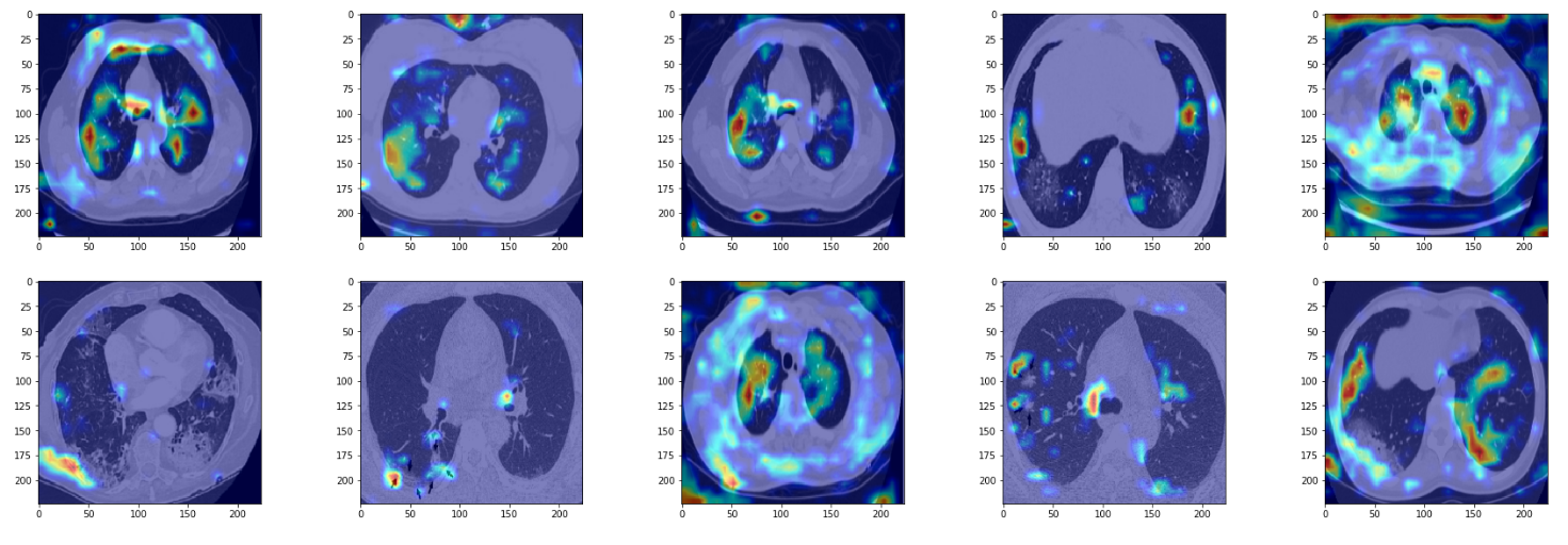
At last, in false negatives, the network is able to pick up on opacities but classifies them as negative. It seems as if the network has some threshold for opacities. In this case, it seems as if the network is thinking of them of as non-COVID pneumonia. In particular, for the images in row 2, col 2 and row 1, col 3, the network has hardly anything to work with.
Another artifact we see is the network focusing on edges of the image, which might be due to overfitting.
Scope for Improvement
While the model does give decent metrics, we can further improve on it. Here are some avenues we can look into.
- Get More Data: At only 746 examples, the dataset is too small for a model trained on it to be deployed in the real world. The model overfits to the dataset, as evident by the TensorBoard log of the accuracies and the losses.
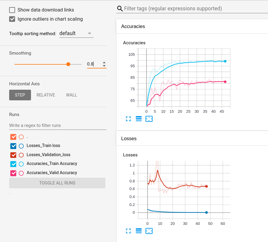
The train accuracy reaches almost 100, whereas the train loss is of the order 0.01. However, the validation accuracy hovers around 80, with validation loss being around 0.6. Adding more data will help. Either one can obtain data, or maybe use GANs to create more medical data, an approach that has been outlined in the following paper.

2. Get Differentiated Data: As I have observed earlier, the data for the negative class is a mix of healthy patients and non-COVID disease sufferers. The performance could be much better if we had labels separating the healthy patients from the non-healthy non-COVID ones. This is perhaps the reason why our model mistakes non-COVID opacities for COVID ones.
3. Use Better Representation: While transfer learning is a very successful technique, performing medical image application on models pretrained on ImageNet, a dataset of everyday items, may not be optimal. Therefore, you might want to learn a representation over some medical task itself. This approach is taken by the authors of the following paper, which achieves a higher accuracy of 86% by using a self contrastive representation learning technique called MoCo to learn a representation over the LUNA16 dataset.

4. Use Better Networks: While we used a vanilla VGG-19, one can use advance architectures to learn the classifier. For example, one paper uses a modification of the Fire module in SqueezeNet and Bayesian optimization to achieve an accuracy of 83%.

While all of these are exciting things to explore, we'll leave these for another post.
Conclusion
In this post we went over creating a simple CNN-based classifier to classify lung CTs as COVID and non-COVID related. We attained an accuracy of 82.8 percent. More than that, this post should provide you with the basic code setup to start experimenting with the COVID-CT dataset so that you can start tinkering with the code to achieve better performance.
A Jupyter Notebook containing all the code can be run for free and downloaded from the ML Showcase.
For more posts related to coronavirus, check out:


