
In the first part of this series on Stock Price Prediction Using Deep Learning, we covered all the essential concepts that are required to perform stock market analysis using neural networks. In this second article, we will execute a practical implementation of stock market price prediction using a deep learning model. The final result obtained might be helpful for users to determine if the outcome of their investments will be worth it in the long term.
Before we dive more deeply into this topic, let us explore the table of contents for this article. This list will help us understand the realistic expectations from this article, and you can feel free to skip to the sections you deem most necessary.
Table of Contents
- Introduction
- Preparing the data
- Visualization of data
- Data pre-processing and further visualization
- Analyzing the data
1. First sets of data elements
2. Second sets of data elements - Building the deep learning model
1. Stacked LSTM model
2. Model summary and plot
3. Compiling and fitting the model
4. Analyzing results - Making Predictions
- Conclusion
Bring this project to life
Introduction
In this article, we will study the applications of neural networks on time series forecasting to accomplish stock market price prediction. You can find the full code for this tutorial and run it on a free GPU from the ML Showcase. While you can directly run the entire notebook on your own, it is advisable that you understand and study each individual aspect and consider code blocks individually to better understand these concepts. The methodology for this project can be extended to other similar applications such as cryptocurrency price predictions as well.
The entire architecture of the stacked LSTM models for the predictive model will be built using the TensorFlow deep learning framework. Apart from the TensorFlow library, we will also utilize other libraries such as pandas, matplotlib, numpy, and scikit-learn for performing various operations throughout the course of the project. These actions include loading and viewing the datasets, visualizing our data, converting it into suitable shapes for computation with stacked LSTMs, and final preparation of before starting our project.
The primary objective of this article is to provide an educative view on the topic of deep learning applications in time series forecasting through the example of stock market price prediction. This example is just one of the many use case options that are available for you to build with neural networks (stacked LSTMs in this case). It is important for to note that before implementing these ideas in real-life scenarios, make sure you explore the numerous tools available to you and check out which ideas work best for your application. Let us now proceed to have a complete breakdown of our project from scratch.
Preparing the data
The first step to complete this project on stock price prediction using deep learning with LSTMs is the collection of the data. We are going to consider a random dataset from Kaggle, which consists of Apple's historical stock data. We are going to read the CSV file using the Panda's library, and then view the first five elements of the data.
# Importing the Pandas Library for loading our dataset
# Grab The Data Here - https://www.kaggle.com/tarunpaparaju/apple-aapl-historical-stock-data

import pandas as pd

df = pd.read_csv('HistoricalQuotes.csv')
df.head()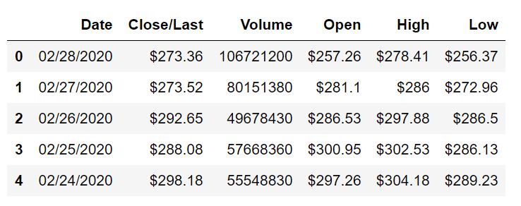
Although there are many parameters to consider for the stock market prediction model, we will only refer to the Close/Last column because it gives us more of an average approach. And it is also easier to consider just one of the columns for training and validation purposes. Keenly observing the dataset is an essential step to solving most Data Science problems. After looking at the dataset, we can easily deduce that the dates are in descending order. We need to correct this.
data = df.reset_index()[' Close/Last'] # Make Sure You add a space
data.head()
Result
0     $273.36
1     $273.52
2     $292.65
3     $288.08
4     $298.18
Name:  Close/Last, dtype: object
Then, we need to arrange our dataset in the ascending order. While you can use the reindex function from the panda's module, I would prefer constructing a new list and reversing that list, and finally creating our new data frame for processing the following tasks.
Option 1
df3 = data.reindex(index=data.index[::-1])
df3.head()
Result
2517     $29.8557
2516     $29.8357
2515     $29.9043
2514     $30.1014
2513     $31.2786
Name:  Close/Last, dtype: object
Option 2
df2 = []

for i in data:
    i = i[2:]
    i = float(i)
    df2.append(i)

df2.reverse()

df1 = pd.DataFrame(df2)[0]
df1.head()
Result
0    29.8557
1    29.8357
2    29.9043
3    30.1014
4    31.2786
Name: 0, dtype: float64
Visualize Your Data
For any machine learning and deep learning problem, one of the most crucial steps is the visualization of your data. Once you visualize and pre-process the data, you can have a brief understanding of the type of model you are dealing with and the necessary steps and measures required to solve the task. One of the best visualization libraries in the Python programming language is the Matplotlib library. It will allow you to visualize the dataset accordingly. Let us plot the model with the data and their respective indexes. The data consists of the values of the stocks at their respective intervals.
# Using the Matplotlib Library for visualizing our time-series data

import matplotlib.pyplot as plt

plt.title("Data Plot")
plt.xlabel("Index")
plt.ylabel("Data")
plt.plot(df1)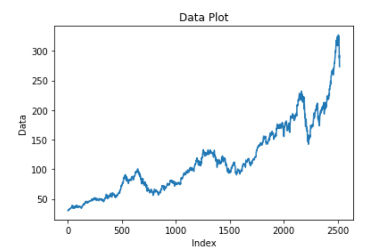
From our visualization, we can notice that the plot of the dollar rate per day usually seems to have an increasing trend.
Data pre-processing and further visualization
Our next steps will be to prepare our dataset. We will import the numpy and scikit-learn libraries for visualizing our data in the form on an array for better modeling. Since the data is a bit large and the values are high, it is better to fit them between 0 and 1 for better computation. We are going to use the Min Max Scaler function from the scikit-learn library to perform the specific action.
import numpy as np
from sklearn.preprocessing import MinMaxScaler

scaler = MinMaxScaler(feature_range=(0,1))
df1 = scaler.fit_transform(np.array(df1).reshape(-1,1))
df1
Result
array([[6.72575693e-05],
       [0.00000000e+00],
       [2.30693463e-04],
       ...,
       [8.83812549e-01],
       [8.19480684e-01],
       [8.18942624e-01]])
From the same sklearn module, we can proceed to import the function to split our data into training and testing datasets. The essential step to consider here is to ensure that the shuffle is set to False because we don't want our data being distributed randomly. Hence, we will give a small test size and distribute the rest to the training data. Once we are done splitting the data as desired, let us proceed to visualize both the train and test datasets that we have created.
from sklearn.model_selection import train_test_split

X_train, X_test = train_test_split(df1, test_size=0.20, shuffle=False)
Training data visualization
plt.title("Data Plot")
plt.xlabel("Index")
plt.ylabel("Data")
plt.plot(X_train)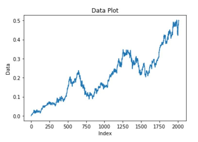
X_train[:5]Result
array([[6.72575693e-05],
       [0.00000000e+00],
       [2.30693463e-04],
       [8.93516807e-04],
       [4.85229733e-03]])
Testing data visualization
plt.title("Data Plot")
plt.xlabel("Index")
plt.ylabel("Data")
plt.plot(X_test)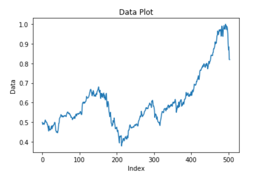
X_test[:5]Result
array([[0.49866208],
       [0.4881699 ],
       [0.49223898],
       [0.49429034],
       [0.49378591]])
Now that we have a brief understanding of how our training and testing data looks like, the next important step is to consider a bunch of these elements and have a prediction for each of them. This procedure is how we will create our final training and testing data along with their respective final training and testing predictions. These predictions or outcomes will be considered as per the timesteps we have considered for our datasets. I will assume a timestep of about 100 data elements and one particular prediction for each of these datasets. This assumption is the integral aspect of time-series analysis with deep learning models.
The elements from the order of 0 to 99 (basically, the first 100 elements) will constitute the elements of the first set of the training or testing dataset. The 100th element will constitute the first prediction. This first outcome will be stored respectively in the results (Y) training or testing list. The next elements from 1 to 100 will constitute the next (or the second) set of elements in the training or testing dataset, while the next prediction or outcome will consist of the 101st element of the dataset. By using this method, we can build our dataset. Our deep learning model architecture will be best suited to solve these kinds of datasets and problems of stock price prediction.
X_train_data = []
Y_train_data = []
X_test_data = []
Y_test_data = []

train_len = len(X_train)
test_len = len(X_test)

# Create the training dataset
for i in range(train_len-101):
    a = X_train[i:(i+100), 0]
    X_train_data.append(a)
    Y_train_data.append(X_train[i + 100, 0])

# Create the test dataset
for j in range(test_len-101):
    b = X_test[j:(j+100), 0]
    X_test_data.append(a)
    Y_test_data.append(X_test[j + 100, 0])

X_train_data = np.array(X_train_data)
Y_train_data = np.array(Y_train_data)
X_test_data = np.array(X_test_data)
Y_test_data = np.array(Y_test_data)
Analyzing The Data
Now that we have a brief understanding of what we are trying to achieve with the previous explanations and code blocks, let us try to gain further insight on this topic by actually analyzing and looking at the first two sets of training data and their respective outputs that are stored in the output dataset.
First set of training data and output
X_train_data[0]Result
array([0.        , 0.00023069, 0.00089352, 0.0048523 , 0.00491451,
       0.00680747, 0.00768182, 0.00799894, 0.00852725, 0.00720127,
       0.00749451, 0.00733578, 0.00759035, 0.00643756, 0.00763844,
       0.00937268, 0.00985794, 0.00855146, 0.01059307, 0.01130902,
       0.0129686 , 0.01256271, 0.0130288 , 0.01423944, 0.01474387,
       0.01525301, 0.01494093, 0.0158247 , 0.01606481, 0.01613206,
       0.01769849, 0.01925013, 0.01851971, 0.01836132, 0.01716985,
       0.02419826, 0.0276812 , 0.02977593, 0.02913699, 0.02555317,
       0.02534164, 0.02872369, 0.02509683, 0.02762369, 0.02393899,
       0.02264428, 0.01796752, 0.012976  , 0.02168586, 0.0229012 ,
       0.02557704, 0.0237853 , 0.02160414, 0.02179616, 0.02090264,
       0.01897134, 0.01388869, 0.01607927, 0.01821234, 0.01747251,
       0.01693882, 0.02137815, 0.02307405, 0.02497173, 0.02647056,
       0.02607206, 0.02263453, 0.02022065, 0.01944719, 0.01650198,
       0.02001383, 0.02145516, 0.02182508, 0.02442425, 0.02805616,
       0.03027566, 0.03133429, 0.02945882, 0.03122668, 0.02984319,
       0.02889688, 0.02779184, 0.02856059, 0.02273306, 0.02050381,
       0.0190386 , 0.01829877, 0.0191109 , 0.02393159, 0.0236555 ,
       0.02439062, 0.02326876, 0.0206326 , 0.02107886, 0.02046547,
       0.01972093, 0.01764536, 0.02067699, 0.02180591, 0.0241041 ])
Y_train_data[0]Result
0.024104103955989345
Second set of training data and output
X_train_data[1]Result
array([0.        , 0.00023069, 0.00089352, 0.0048523 , 0.00491451,
       0.00680747, 0.00768182, 0.00799894, 0.00852725, 0.00720127,
       0.00749451, 0.00733578, 0.00759035, 0.00643756, 0.00763844,
       0.00937268, 0.00985794, 0.00855146, 0.01059307, 0.01130902,
       0.0129686 , 0.01256271, 0.0130288 , 0.01423944, 0.01474387,
       0.01525301, 0.01494093, 0.0158247 , 0.01606481, 0.01613206,
       0.01769849, 0.01925013, 0.01851971, 0.01836132, 0.01716985,
       0.02419826, 0.0276812 , 0.02977593, 0.02913699, 0.02555317,
       0.02534164, 0.02872369, 0.02509683, 0.02762369, 0.02393899,
       0.02264428, 0.01796752, 0.012976  , 0.02168586, 0.0229012 ,
       0.02557704, 0.0237853 , 0.02160414, 0.02179616, 0.02090264,
       0.01897134, 0.01388869, 0.01607927, 0.01821234, 0.01747251,
       0.01693882, 0.02137815, 0.02307405, 0.02497173, 0.02647056,
       0.02607206, 0.02263453, 0.02022065, 0.01944719, 0.01650198,
       0.02001383, 0.02145516, 0.02182508, 0.02442425, 0.02805616,
       0.03027566, 0.03133429, 0.02945882, 0.03122668, 0.02984319,
       0.02889688, 0.02779184, 0.02856059, 0.02273306, 0.02050381,
       0.0190386 , 0.01829877, 0.0191109 , 0.02393159, 0.0236555 ,
       0.02439062, 0.02326876, 0.0206326 , 0.02107886, 0.02046547,
       0.01972093, 0.01764536, 0.02067699, 0.02180591, 0.0241041 ])
Y_train_data[1]Result
0.024544304746736592
As the final step of our analysis and pre-processing, let us print the shapes of our training and testing dataset as well as their respective outputs. The shapes of the training and testing datasets must contain 100 elements in each of their sets, while their respective results must have the shape equivalent to the number of sets present in the training or testing datasets. Using these figures and shapes, we can finally proceed to the final step of our pre-processing.
### Printing the training and testing shapes

print("Training size of data = ", X_train_data.shape)
print("Training size of labels = ", Y_train_data.shape)
print("Training size of data = ", X_test_data.shape)
print("Training size of labels = ", Y_test_data.shape)
Result
Training size of data =  (1913, 100)
Training size of labels =  (1913,)
Training size of data =  (403, 100)
Training size of labels =  (403,)
Now that we have a brief idea of the shapes produced by our testing and training datasets as well as their respective outputs, the final essential step is to convert these existing shapes of the datasets into a form suitable for Long short-term memory (LSTM) models. Since our current structure is only a 2-dimensional space, we need to convert it into a 3-dimensional space for making it suitable to perform LSTM operations and computations.
### Converting the training and testing data shapes into a 3-dimensional space to make it suitable for LSTMs

X_train_data = X_train_data.reshape(1913, 100, 1)
X_test_data = X_test_data.reshape(403, 100, 1)

print(X_train_data.shape)
print(X_test_data.shape)
Result
(1913, 100, 1)
(403, 100, 1)
Building The Deep Learning Model
We will be using the stacked LSTM layers and build our deep learning neural network to construct an architecture to encounter this task. Firstly, we will import all the essential libraries for performing this computation. We will be using a simple Sequential architecture. I would highly recommend checking out my previous two articles on the introduction to TensorFlow and Keras to learn a more detailed approach to these specific topics.
 Bharath K
 Bharath K
However, to provide a short summary on these topics, a Sequential model is one of the simplest architectures to build your deep learning models and construct your neural networks for solving a variety of complex tasks. A Sequential model is appropriate for a plain stack of layers where each layer has exactly one input tensor and one output tensor.
The only two layers that we will require for processing our computation of the stock market price prediction problem are the Dense layers and the LSTM layers. The Dense layers basically act like a fully connected layer in a neural network. They can be used either as hidden layers with a specific number of nodes or as an output layer with a specific number of nodes. Here, our Dense layer will only have one output node because we only require one output or prediction for a specific set of parameters or sets of data. We have already discussed in further detail the topic of LSTM layers previously.
from tensorflow.keras.models import Sequential
from tensorflow.keras.layers import Dense
from tensorflow.keras.layers import LSTM

# Build The Architecture

model=Sequential()
model.add(LSTM(100,return_sequences=True,input_shape=(100,1)))
model.add(LSTM(100,return_sequences=True))
model.add(LSTM(100))
model.add(Dense(1))
With that step complete, we have finished building our stack LSTM architecture that we can utilize for making stock market predictions. However, we still have a few steps left before the model can be deployed and used to make actual predictions and find out the outcome. Let us look into the model summary and the model plot.
model.summary()Result
Model: "sequential"
_________________________________________________________________
Layer (type)                 Output Shape              Param #
=================================================================
lstm (LSTM)                  (None, 100, 100)          40800
_________________________________________________________________
lstm_1 (LSTM)                (None, 100, 100)          80400
_________________________________________________________________
lstm_2 (LSTM)                (None, 100)               80400
_________________________________________________________________
dense (Dense)                (None, 1)                 101
=================================================================
Total params: 201,701
Trainable params: 201,701
Non-trainable params: 0
_________________________________________________________________
Model Plot
# Plot the Model

from tensorflow import keras
from keras.utils.vis_utils import plot_model

keras.utils.plot_model(model, to_file='model.png', show_layer_names=True)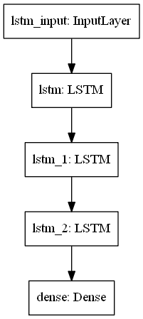
Before we move on to the compilation and training procedures, I will implement one callback that will be useful for saving our checkpoints for the best value of validation loss processed. The reason for saving the best models is so that you can use them later on to load these models and choose to make further predictions with the saved models. While you are simply loading the models as required, you do not have to repeat the entire procedure of training and fitting again repeatedly. During the deployment stages, the saved model can be used for making further predictions.
The second and final callback that we will utilize for our model is the tensorboard callback. We will mainly use the tensorboard callback from the Keras module for visualizing the graphs of the training loss and the validation loss. We will be using a random log directory that will store the folders for the training and validation data. Finally, we will utilize this directory with the Tensorboard callback function. Once our training is complete, we can utilize this saved information from the logs directory to visualize our training and validation losses.
You can also use other callbacks, as mentioned in my previous Keras article. However, I do not deem it necessary to use any of the other Keras or custom callbacks for performing this specific task. You can feel free to try out the other callbacks if you want to explore them in further detail.
# Initializing the callbacks

from tensorflow.keras.callbacks import ModelCheckpoint
from tensorflow.keras.callbacks import TensorBoard

checkpoint = ModelCheckpoint("checkpoint1.h5", monitor='val_loss', verbose=1,
                              save_best_only=True, mode='auto')

logdir='logs1'
tensorboard_Visualization = TensorBoard(log_dir=logdir)
After initializing our callbacks, we can proceed to compile the stacked LSTM model that we completed building using the Sequential modeling architecture. The loss function we will utilize for the compilation of the model is the mean squared error. The mean squared error function computes the mean of squares of errors between labels and predictions. The formulation of the equation is interpreted as follows:
$loss = square(y_true - y_pred)$
As discussed previously in my Keras article, one of the best optimizers to choose by default for performing the compilation of the model is the Adam optimizer. Adam optimization is a stochastic gradient descent method that is based on an adaptive estimation of first-order and second-order moments. You can also feel free to try out other optimizers such as RMS Prop and see if you are able to achieve better results during the training procedure.
# Model Compilation

model.compile(loss='mean_squared_error', optimizer='adam')
The final step after the construction and compilation of the model is to train the model and ensure the fitting process occurs perfectly. During the training stage, we will use the fit function of our model and then train both the X_train (the training data) as well as the X_test (Validation data) accordingly. Make sure you give the equivalent parameters accordingly. The first two attributes in the fit function should have the training data and their predictions, respectively. For the next parameters, we will ensure that we compute the validation data consisting of the test data and their predictions, respectively enclosed in parentheses.
I will be running the model for twenty epochs. You can choose to run it for more than the specified epochs if you want to obtain a slightly better result. I will use a batch size of 32 for the fitting process, but if you are increasing the number of epochs, you can also feel free to edit this in the form of increasing batch sizes like 64, 128, etc. The verbose parameter, when set as 1, will allow you to see the training procedure occurring in each step. You can also choose to set it as 0 or 2, as per your convenience. Finally, we will implement the callbacks function that consists of our previously defined callbacks. Now that we have completed defining all the required parameters for the fit function, we can run the code block and observe the training process.
# Training The Model

model.fit(X_train_data,
          Y_train_data,
          validation_data=(X_test_data, Y_test_data),
          epochs=20,
          batch_size=32,
          verbose=1,
          callbacks=[checkpoint, tensorboard_Visualization])
Result
Epoch 19/20
1824/1913 [===========================>..] - ETA: 0s - loss: 1.0524e-04
Epoch 00019: val_loss improved from 0.04187 to 0.03692, saving model to checkpoint1.h5
1913/1913 [==============================] - 1s 508us/sample - loss: 1.0573e-04 - val_loss: 0.0369
Epoch 20/20
1824/1913 [===========================>..] - ETA: 0s - loss: 1.3413e-04
Epoch 00020: val_loss did not improve from 0.03692
1913/1913 [==============================] - 1s 496us/sample - loss: 1.3472e-04 - val_loss: 0.0399
Tensorboard Analysis
After the execution of the fitting code block, we will have a saved checkpoint labeled as "checkpoint1.h5", using which we can directly load the best weights of our model and start making predictions with it directly. There is no need to re-train the entire model once again.
We will now refer to the working environment once again to notice that we can find a newly created directory called logs1. The logs1 directory consists of the training and validation events that will be utilized by us to understand and analyze the training and validation components. The graphs produced will give us a brief description and understanding of the performance of the loss and validation loss with the increasing epochs. To access these graphs, open a command prompt in your respective workspace and type the following command after activating your respective virtual environment - tensorboard --logdir="./logs1".
After the execution of the following, you should be able to access your localhost from your web browser, which should direct you to the tensor board graphs that you can view. Let us now proceed to analyze the training and validation loss graphs.
from IPython.display import Image

pil_img = Image(filename='image1.png')
display(pil_img)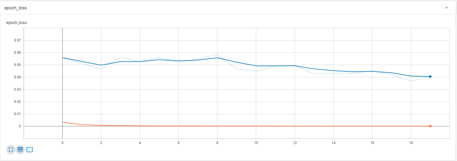
Since the tensor board graph does not appear to give us the precise required value in the first image, let us scale in a bit and zoom into it a bit more so that we can analyze the values a bit more closely.
pil_img = Image(filename='image2.png')
display(pil_img)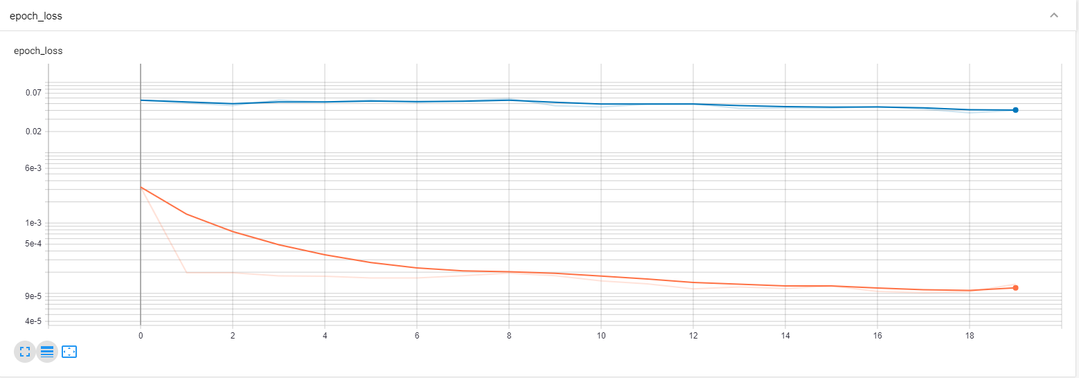
From the second image, it is clearly visible that both the training loss and validation loss are decreasing with increasing epochs. Hence, we can determine that the fitting procedure of the model is working pretty well because the model is constantly improving with the increasing number of epochs.
Predictions and Evaluations
In the next few code blocks, we will use the predict function from the model to make the respective predictions on the training and testing data. It is essential to note that we had previously converted the range of values for the training and testing data from 0 to 1 for faster and efficient computation. Hence, it is now time to use the inverse transform attribute from the scaler function to return the desired values. By making use of this procedural method, we will achieve the required result that we need to attain since the values obtained are scaled back to their original numbers.
We will also analyze the Mean Square Error (MSE) parameters for both the training and testing data. The method for performing this task is fairly simple. We will require two additional libraries, namely math and sklearn.metrics. From the metrics module, we will import the mean squared error function that will help us to compute the mean squared error between the training values and testing values with their respective predictions effectively. Once we have computed, calculated, and acquired the required MSE values, we can determine that the root of these MSE values is not too bad and are able to produce effective results. They are compatible with the model built and can be used to make decent and appropriate predictions.
train_predict = model.predict(X_train_data)
test_predict = model.predict(X_test_data)

# Transform back to original form
train_predict = scaler.inverse_transform(train_predict)
test_predict = scaler.inverse_transform(test_predict)
# Calculate RMSE performance metrics for train and test data
import math
from sklearn.metrics import mean_squared_error
print("Train MSE = ", math.sqrt(mean_squared_error(Y_train_data, train_predict)))
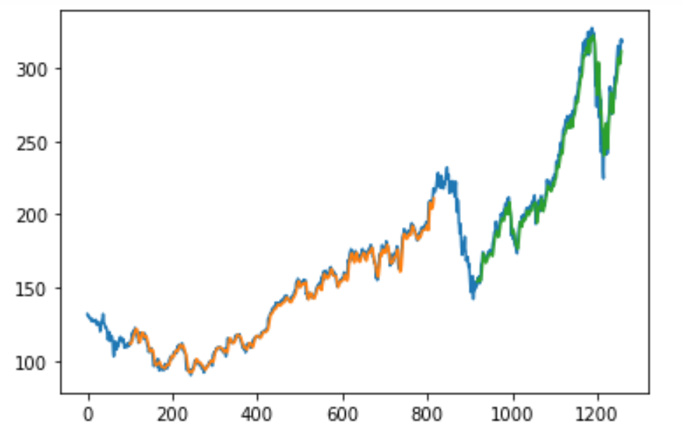
print("Test MSE = ", math.sqrt(mean_squared_error(Y_test_data, test_predict)))Finally, we will evaluate our model and analyze the numerous parameters. A small reference for the code is considered from here. I would recommend checking the following website as well to gain further information on this topic. For further detail on how you can build the predictive systems to evaluate and test your model, you can check out this link. The below graphical structure is an example and a brief representation of the type of graph that we will obtain when we try to make the respective predictions. Feel free to try these methods on your own from the provided references. I will not be covering them in this article because the intended purpose is to only provide an educational perspective and view on these concepts.
With this, we have successfully built our stock market prediction model with the help of LSTMs and Deep Learning.
Conclusion
We have completed our construction of the stacked LSTM deep learning model that finds its uses in fields of stock market price prediction, cryptocurrency mining and trends, and numerous other aspects of daily life. You can even build similar models to understand everyday weather patterns and so much more. The field of time-series forecasting with deep learning is humungous to explore. It provides a wide variety of opportunities for us to work on many different kinds of unique projects and construct deep learning models. These deep learning models built will create an amazing approach for us to contemplate the working of many time-series problems.
The previous article addressed most of the common topics related to time-series forecasting. Please check out part-1 of this series to understand most of the concepts more intuitively. The first part provides a conceptual overview of the knowledge required for some of the essential topics of time-series forecasting, as well as includes some of the theoretical explanations to the content covered in this second part. With the help of the Jupyter Notebook provided in this article, feel free to explore and try out a variety of integrations to improve the performance of the model and create much more innovative projects.
Thank you all for reading this 2-part series. In future articles, we will cover more topics on GANs, forecasting, NLP models, and so much more. Until then, enjoy coding and keep up the practice!