
In the first part of this article on Stock Price Prediction Using Deep Learning, we will master most of the topics required to understand the essential aspects of forecasting and time-series analysis with machine learning and deep learning models. Time series analysis (or forecasting) is growing to be one of the more popular use cases of machine learning algorithms in the modern era. To understand the different types of patterns in the analysis of the time series, and to determine a realistic future prediction, our machine learning or deep learning models need to be trained appropriately.
In this article, our primary objective will remain on understanding all the essential tools and core concepts for solving problems related to time series analysis and forecasting. In the second and final part of this series, we will cover a complete and intuitive example of how you can build your own stock market price prediction model from scratch (namely a stacked LSTM model). For now, let's look at the table of contents to set your expectations for Part 1.
Table Of Contents
- Introduction
- Why do we require time series analysis?
- Essential components of time series analysis
1. Trend
2. Seasonality
3. Irregularity
4. Cyclic - Understanding stationary and non-stationary series
- Understanding LSTMs in detail
- When not to use time series analysis
- Conclusion
Bring this project to life
Introduction
Most of the natural events that occur in the world have some amount of time series forecasting involved in them. The primary object of time-series forecasting is one variable, which is time. Time series data analysis is useful for the extraction of meaning statistics and other important characteristics.
Time series analysis involves the sequential plotting of a set of observations or data points at regular intervals of time. By studying previous outcomes and their progression over time, we can make future predictions with the help of these studied observations.
The approach to problems related to time series analysis is unique in its own way. Most machine learning problems utilize a dataset with certain outcomes to be predicted, such as class labels. This statement means that most machine learning tasks usually utilize an independent and dependent variable for the computation of a particular question.
This procedure involves machine learning algorithms analyzing a dataset (say, $X$) and using the predictions ($Y$) to form an assessment and approach to solving the problem statement. Most supervised machine learning algorithms perform in this manner. However, time series analysis is unique because it has only one variable: time. We will dive deeper into how to solve the stock market price prediction task with deep learning in the next part of this article. For now, our primary objective will be understanding the terms and important concepts required for approaching this task. Let us begin!
Why do we require time series analysis?
The ordered sequence of data points in regular intervals of time constitutes the primary elements of time series analysis. Time series analysis has a wide range of applications in the practical world. Hence, the study of time series is significant to understand, or at the very least, to gain basic knowledge about what you can expect in the near future. Apart from the stock market price prediction model that we will build in the next part of these articles, time series analysis has applications in economic forecasting, sales forecasting, budgetary analysis, process and quality control, detection of weather patterns, inventory and utility studies, and census analysis, among many others.
Understanding previous behavioral patterns of data elements is critical. Consider an example of business or economic forecasting. When you can extract useful information from the previous patterns, you can plan the future accordingly. More often than not, the predictions made with the help of time series analysis and forecasting yield good results. These will help users to plan and evaluate current accomplishments.
Essential components of time series analysis
Time series analysis is all about the collection of previous data to study the patterns of various trends. By conducting a detailed analysis of these time series forecasting patterns, we can determine the future outcomes with the help of our constructive deep learning models. While there are other methods to determine the realistic results of future trends, deep learning models are an outstanding approach to receive some of the best predictions for each concept.
Let's now focus on the components of time series forecasting, namely Trend, Seasonality, Cyclicity, and Irregularity. These four components of time series analysis refer to types of variations in their graphical representations. Let us look at each of these concepts individually and try to gain more intuition behind them with the help of some realistic examples.
Trend
A Trend in time series forecasting is defined as a long period of time with a consistent increase or decrease in the data. There may be slight fluctuations in the data points and elements at various instances of time, but the overall variation and direction of change remain constant for a longer duration of time. When a Trend goes from a long duration of constant increase to a long duration of constant decrease, this is often referred to as a "Changing Direction" trend.
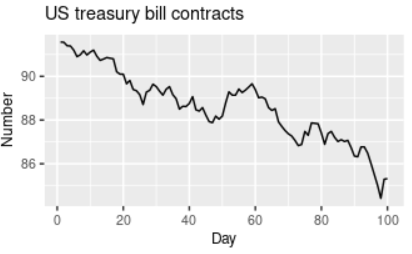
There a few terminologies used to define the type of trend that we are dealing with in time series forecasting. A slightly or moderately increasing trend over a long duration of time can be referred to as an uptrend, while a slightly or moderately decreasing trend over a long duration of time is called a downtrend. If the trend is following a consistent pattern of gradually increasing or gradually decreasing, and there is not much effect in the overall pattern of the graph, then this trend can be referred to as a horizontal or stationary trend. The graphical representation shown in the above image has a downward trajectory over a long period of time. Hence, this image shows the representation of a downward trend, also called a downtrend.
Let us consider an example to understand the concept of trend better. Successful companies like Amazon, Apple, Microsoft, Tesla, and similar tech giants have a reasonably performing upward stock price curve. We have learned that we can determine this upward rise in stock prices as an uptrend. While successful companies have an uptrend, some companies that are not performing that well in the stock market have downward trajectories in stock prices, or a downtrend. Companies that are making a neutral profit rate with decent amounts of profits and losses at regular intervals are determined as a horizontal or stationary trend.
Seasonality
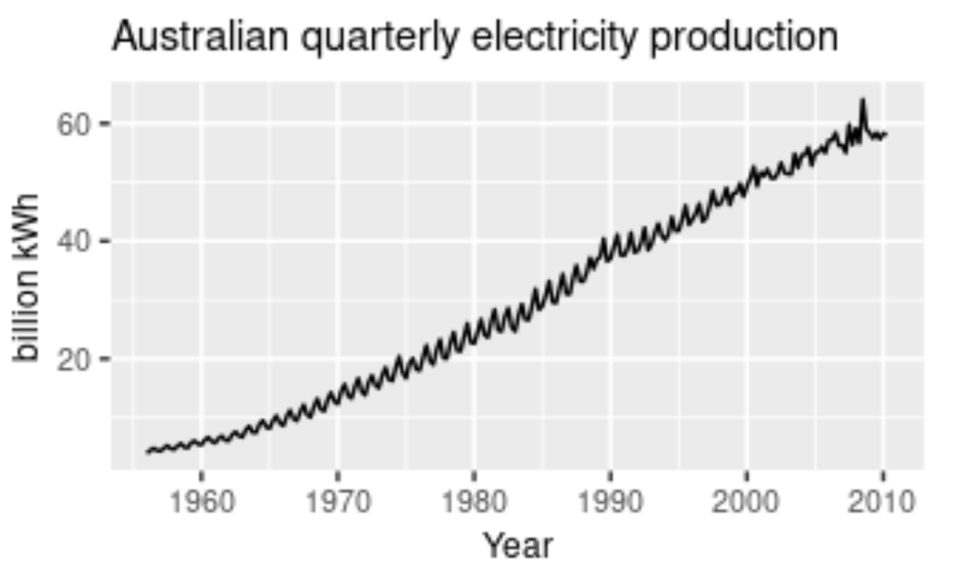
A pattern that is affected or influenced by seasonal frequency variations are termed to be seasonal. This component of time series analysis can vary from time stamps like quarterly, monthly, or half-yearly. However, an important point to note is that these fluctuations usually take place within the period of a year. Whenever the frequency is fixed and known and also occurs on a timely basis, usually within a year, this component of time series analysis is known as seasonality.
To consider a realistic example, think about the sale of certain seasonal fruits. Fruits like watermelon will have increased sales during the summer season, while during the winter seasons, the sales of watermelons will gradually reduce. Similarly, seasonal fruits like apple have higher sales during the winter seasons in comparison to the other seasons. Ice cream and tender coconuts are other examples of food products that have increased sales during the summer season while experiencing a dip in sales during other seasons. Apart from food products, a period or month like April might have higher shares of investment and experience a dip in shares until six months later in October, where it has a peak rise. This pattern can also be regarded as a seasonality.
Cyclicity
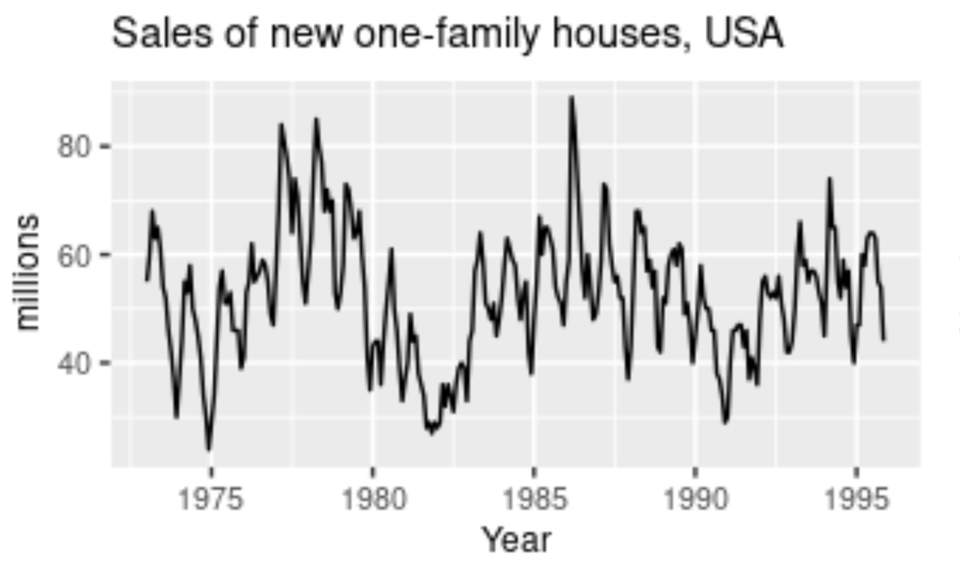
When a pattern exhibits a rise and fall of mixed frequencies, and the graphical representation has peaks and troughs that occur randomly over a period of time, it is called a cyclic component. The duration of these occurrences usually ranges over the period of at least one year. Stock prices of certain companies that are hard to predict usually have cyclic patterns where they flourish during a certain period, while having lower profits at other times. Cyclic trends are some of the hardest for our deep learning models to predict. The graphical representation above shows the cyclic behavior of house sales over the span of two decades.
A great realistic example of cyclic behavioral patterns is when a person decides to invest in their own start-up. During the set-up and progression of start-ups, every business experiences a cyclic phase. These cyclic fluctuations often occur in business cycles. Usually, the phases of a start-up would include the investment stage, which would have a slightly negative impact on our prices. The next phases could include your marketing and profitable stages, where you start to earn profits from your successful start-up. Here, you experience an increase in the graphical curve. However, you will eventually experience a depreciation phase as well. These will show lesser profits until you make constant improvements and investments. This procedure begins the cyclic stage again, lasting for periods of a few years. Rinse and repeat.
Irregularity
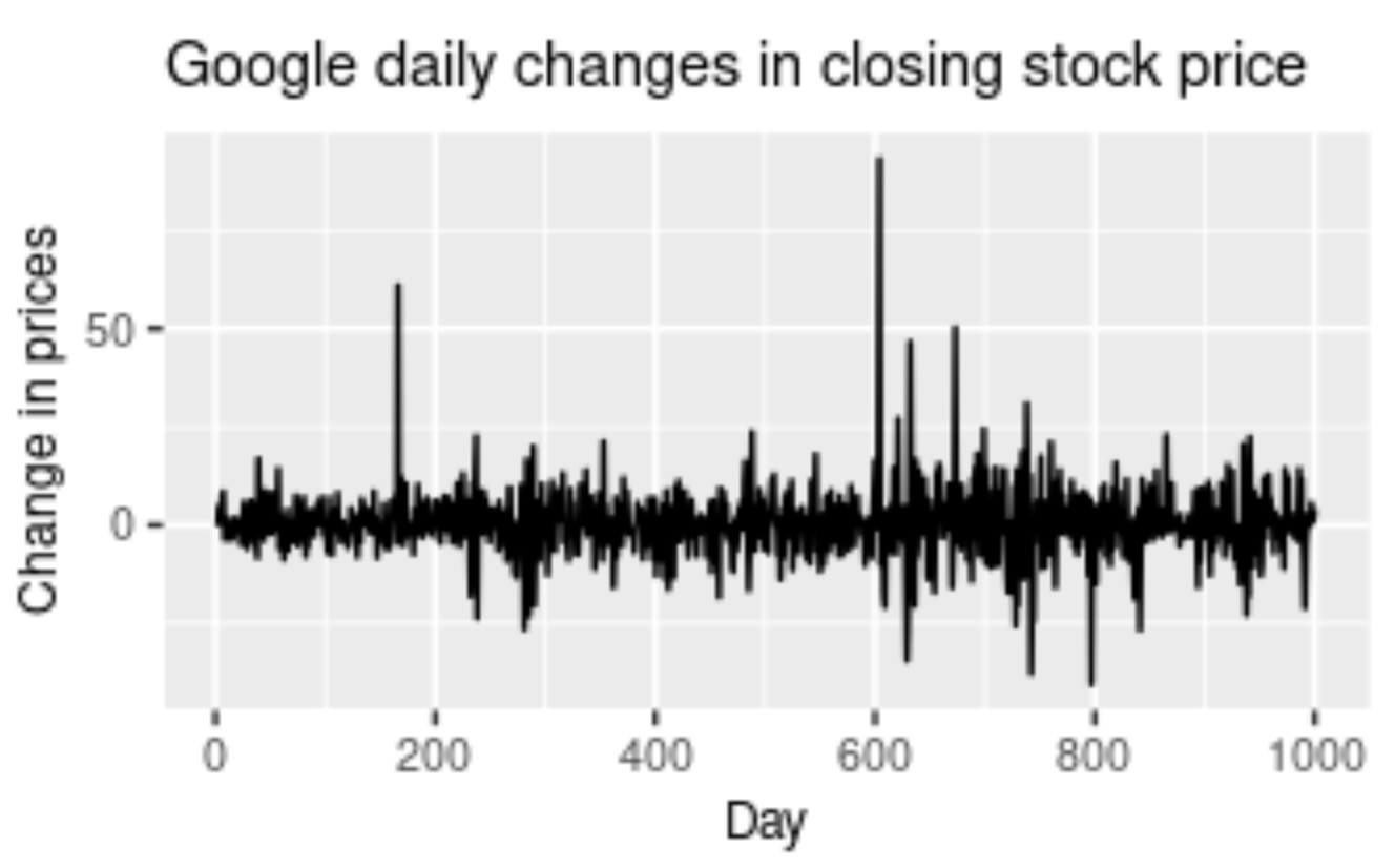
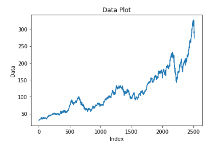
Irregularity is a component that is almost impossible to make accurate predictions for with a deep learning model. Irregularity, or random variations (as the name suggests), involves an abnormal or atypical pattern where it becomes hard to deduce the occurrences of the data elements with respect to time. Above is a graphical representation of the Google Stock Price changing rapidly with an irregular and random pattern; this is hard to read. Despite the information and data patterns present, the modeling procedure for such kinds of representations will be hard to crack. The primary objective of the model is to predict future possibilities based on previous outcomes. Hence, models for irregular patterns are slightly harder to construct.
To provide a realistic example for irregular patterns, let us analyze the current status of the world, where many businesses and other industries are affected on a large scale. The global pandemic is a great example of irregular activity that is impossible for anyone to predict. These disturbances that occur due to a natural calamity or phenomenon will affect the trading prices, stock price charts, companies, and businesses. It is not possible for the model you construct to detect the occurrences of these situational tragedies. Hence, irregular patterns are an interesting component of time series forecasting to analyze and study.
Understanding stationary and non-stationary series
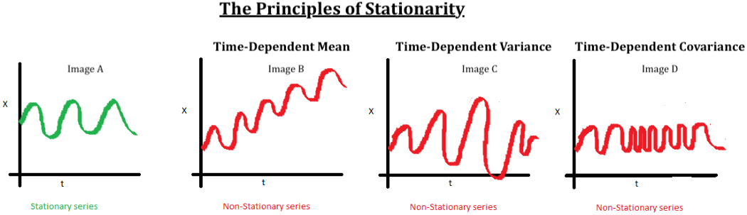
Another significant aspect of time series analysis that we will encounter in this article is the concept of stationarity. When we have a certain number of data points or elements, and the mean and variance of all these data points remain constant with time, then we call it a stationary series. However, if these elements vary with time, we call it a non-stationary series. Most forecasting tasks, including stock market prices or cryptocurrency graphs, are non-stationary. Unfortunately, the results obtained by non-stationary patterns are not efficient. Hence, they need to be converted into a stationary pattern.
The entire data preparation process for stock market price prediction in the next article is explained with code snippets. Here, we will discuss a few other topics of importance. Several methods for converting non-stationary series into stationary series include differencing and transformation. Differencing involves subtracting two consecutive data points from the higher to lower order, while transformation involves transforming or diverging the series. Typically, a log transform is used for this process. For further information on this topic, refer to the link provided in the image source above.
To test for stationarity in Python, the two main methods that are utilized include rolling statistics and the ADCF Test. Rolling statistics are more of a visual technique that involves plotting the moving average or moving variance to check if it varies with time. The Augmented Dickey-Fuller test (ADCF) is used to give us various values that can help in identifying stationarity. These test results comprise some statistics and critical values. They are used to verify stationarity.
Let us now proceed to understanding the concept of LSTMs for time series analysis in detail.
Understanding LSTMs in detail
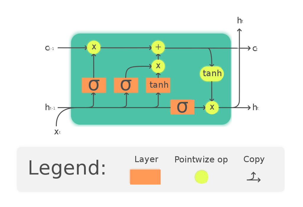
Recurrent neural networks, also known as RNNs, are a class of neural networks that allow previous outputs to be used as inputs while having hidden states. The more in-depth details pertaining to RNNs will be covered in a future article. The primary focus and objective here will remain on studying and gaining a better intuition on LSTM architectures. RNNs have issues with the transfer of long-term data elements due to the possibility of exploding and vanishing gradients. The fix to these issues is offered by the Long short-term memory (LSTM) model, which is also a recurrent neural network (RNN) architecture that is used to solve many complex deep learning problems. LSTMs are especially useful for our task of Stock Price Prediction Using Deep Learning.
The LSTM architecture, with its effective mechanism of memory cells, is extremely useful for solving complex problems and making overall efficient predictions with higher accuracy. LSTMs learn when to forget and when to remember the information provided to them. The basic anatomy of the LSTM structure can be viewed in three main steps. The first stage is the cell state that contains the basic and initial data to be recollected. The second stage is the hidden state that consists of mainly three gates: the forget gate, input gate, and output gate. We will discuss these gates shortly. Finally, we have a looping stage that reconnects the data elements for computation at the end of each time step.
One time step is said to be completed once all the states are updated. Let us explore the concept of gates and decipher the purpose of each of them.
- Forget Gate: One of the most essential gates in LSTMs that utilize the sigmoid function to choose which values to keep or throw away. Values closer to 1 are usually kept while the values closer to 0 are neglected.
- Input Gate: The input gate serves the purpose of deciding what to add to the LSTM cells. It utilizes both the sigmoid and tanh functions. The tanh functions squeeze the values between -1 and 1 to prevent the values from becoming too large on either spectrum.
- Output Gate: The output gate decides the components of the next hidden state. It is also the overall compilation of the entire LSTM structure.
Below is a simple code representation of a stacked LSTM structure that will be utilized for computation purposes in the next part of this series. The block of code is written with the TensorFlow deep learning framework with the help of the Sequential model architecture.
model.add(LSTM(100,return_sequences=True,input_shape=(100,1)))
model.add(LSTM(100,return_sequences=True))
model.add(LSTM(100))
The mathematical computations for LSTMs can be interpreted in many ways. The images shown below are two of the methods in which the mathematical calculations of LSTMs are carried out. Sometimes the bias function is ignored, as shown in the second image. However, we will not cover the intricate details of the first image. You can check out more on that representation from the link provided in the image source. The mathematical equations in consideration of the first LSTM image are pretty accurate for computation purposes.
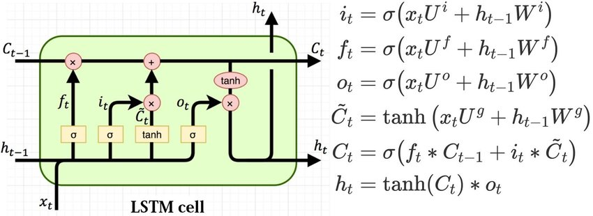

Where:
• $X(t)$: input vector to the LSTM unit
• $F(t)$: forget gate's activation vector
• $I(t)$: input/update gate's activation vector
• $O(t)$: output gate's activation vector
• $H(t)$: hidden state vector, also known as output vector of the LSTM unit
• $c̃(t)$: cell input activation vector
• $C(t)$: cell state vector
• $W$, $U$,and $B$: weight matrices and bias vector parameters which need to be learned during training
For further information and exploration on the topic of Long short-term memory (LSTM), I would highly recommend checking out a few articles that cover this concept extensively. My main two recommendations would be to check out the official documentation of Wikipedia that contains most of the theoretical information for learning about LSTMs. The second link you should check out for a more intuitive understanding is here. Let us now proceed to understand a few cases where the use of time series analysis may be unnecessary or even detrimental.
When not to use time series analysis
From the previous sections of this article, it has become evident that time series forecasting is a valuable asset in today's world. The applications of time series analysis are widespread, and there are a variety of use cases in our daily life. In spite of these facts, there are also certain scenarios where you are better off without the utilization of forecasting. Below are two such scenarios.
The values are constant in the analytic patterns
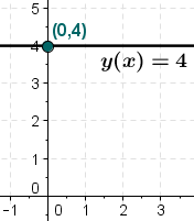
When the values are constant, the whole point of applying time series forecasting becomes futile. You will always have a fixed constant value no matter what the external variations are changed to. Hence, such scenarios do not require the involvement of time-series analysis. The above graphical representation is an example of a constant graph, where the values remain fixed at four no matter what the other constraints are. To consider a real-life example, you can assume the cost of any particular chocolate that remains unchanged over a long period of time.
The values available in the analytic pattern are in the form of functions
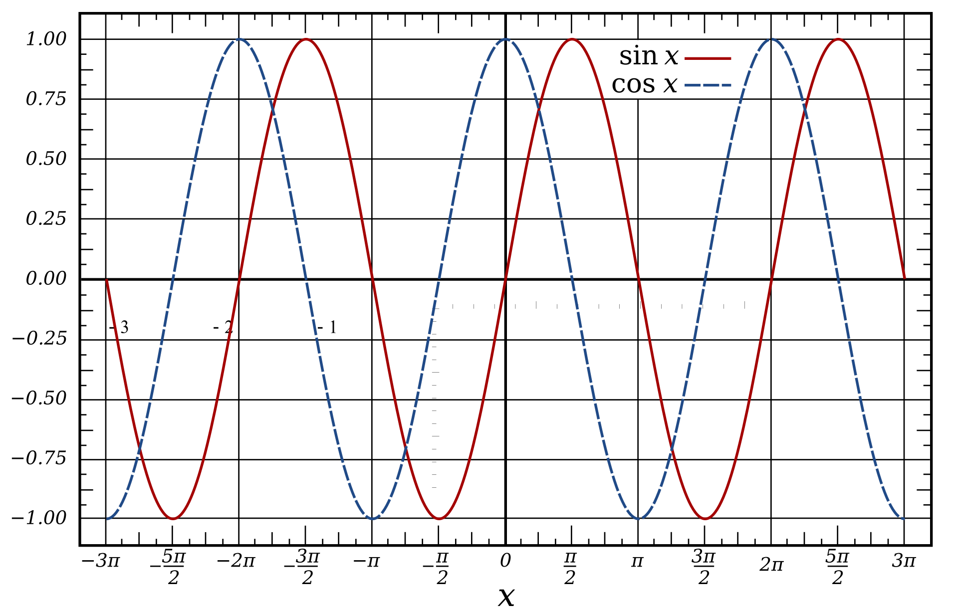
Similar to the previously discussed point, when there is a fixed function that has the required values for each desirable point of time, then the whole point of time series forecasting is nullified. When the time series analysis is in the form of a function, the mathematical calculation for this pattern could be done with a calculator. To consider some such examples, the above graph shows the representation of a sine and cosine wave. Any function of the form $Y(x) = X$ is simple enough to calculate, and we don't need deep learning to do so.
Conclusion
In this article, we have covered most of the basic and essential requirements for dealing with problems related to time series forecasting. The most significant topic covered was Long Short-Term Memory (LSTM). LSTM will be utilized for the stock price prediction project we will build in the next tutorial.
In our next article, we will work on the project of stock market price prediction using deep learning, namely stacked LSTMs. We will prepare the dataset, visualize the data points, and build out our model structure. Feel free to check out my previous couple of articles and gain an intuitive understanding of deep learning frameworks such as TensorFlow and Keras from the links provided below. These libraries will be required for us to work on our project.
 Bharath K
 Bharath K
It is highly recommended that you check out the guides to these libraries as they will be used extensively in the second part of our article series. The next part will contain the complete walkthrough. Until then, strengthen your basics and prepare yourself for the next article!


