The Absolute Guide to TensorFlow

TensorFlow is one of the most popular deep learning libraries of the modern era. Developed by Google and released in 2015, TensorFlow is considered to be one of the best platforms for researching, developing, and deploying machine learning models.

The core structure of TensorFlow is developed with programming languages such as C and C++, which makes it an extremely fast framework. TensorFlow has its interfaces available in programming languages like Python, Java, and JavaScript. The Lite version also allows it to be run on mobile applications, as well as embedded systems.

In this tutorial we'll break down the most essential aspects of TensorFlow and Keras while programming deep learning models with these modules.

Table of Contents

• Introduction to TensorFlow and Keras
• Accelerators
  1. CPUs
  2. GPUs
  3. TPUs
• Quick Starter Guide for Beginners
• Basic Functionalities and Operations
  1. Tensors
  2. Constants and Variables
  3. Backpropagation
  4. Graphs
  5. Introduction to Layers and Models
• Understanding TensorFlow 2.x
  1. Gradient Clipping
  2. Gradient Reversal
  3. Gradient Tape
• Conclusion

You can follow along with the complete code in this tutorial and run it for free from a Gradient Community Notebook.

Introduction to TensorFlow and Keras

TensorFlow uses a low-level control-based approach, with intricate details required for coding and developing projects, resulting in a steeper learning curve.

This is where Keras comes into the picture!

Keras was originally developed by various members of the Google AI team. The first version of Keras was committed and released on GitHub by the author François Chollet on March 27th, 2015.

Keras is a simple, high-level API that works as a front-end interface, and it can be used with several backends. Up until version 2.3, Keras supported various deep learning libraries like TensorFlow, Theano, Caffe, PyTorch, and MXNET. However, with the most stable version Keras 2.4 (released on 17th June 2020), only TensorFlow is now supported.

When TensorFlow was initially released, Keras was just one of the popular high-level APIs that could be used with it. With the release of TensorFlow 2.0, Keras is now integrated with TensorFlow and is considered the official high-level TensorFlow API for quick and easy model design and training.

Accelerators

Deep learning involves a lot of complex computations to achieve desirable results. One of the main reasons for the failure of deep learning and neural networks a few decades ago was due to a lack of sufficient data, as well as a shortage of advanced computational technologies.

However, in the modern generation, the abundance of data and continuous progressions in technology have resulted in deep learning emerging as a powerful tool to solve complicated problems such as face recognition, object detection, image segmentation, and so many other complex tasks.

In this section, we will discuss an essential aspect of deep learning that involves boosting the functionality of deep learning libraries like TensorFlow: the accelerators. The AI accelerator is a class of specialized hardware accelerator, i.e. a computer system designed to accelerate Artificial Intelligence applications, namely in the fields of Machine Learning, Computer Vision, Natural Language Processing, and IoT applications, among others.

Let's analyze a few common tools that are used for processing. The most commonly used accelerators can be categorized as follows.

CPUs

The simplest (and default) way to run the TensorFlow deep learning library on your local system is with the Central Processing Unit (CPU). The CPU has a few cores generally ranging from 4–12, which can be used to compute the calculations pertaining to deep learning tasks (like the backpropagation computations).

However, the CPU is only a basic, simple accelerator that cannot perform many operations in parallel. The CPU version of TensorFlow can be used to solve simple tasks in a short amount of time. But, with an increase in the size of the model architecture, number of nodes, and trainable parameters, the CPU is extremely slow and may even be unable to handle the processing load.

GPUs

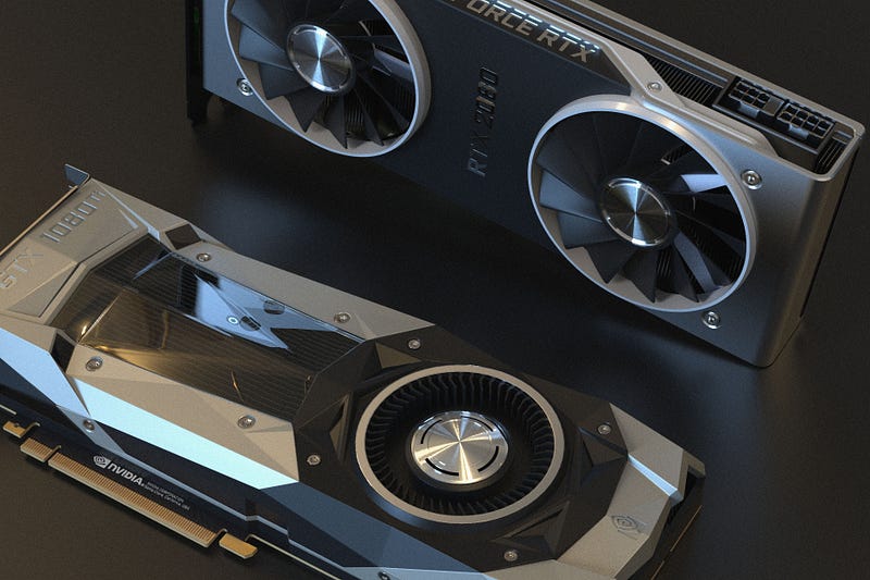
Graphics Processing Units (GPUs, or graphics cards) have revolutionized deep learning. These accelerators can be integrated with the Tensorflow-GPU version to implement various operations and tasks.

NVIDIA provides something called the Compute Unified Device Architecture (CUDA), which is crucial for supporting various deep learning applications. CUDA is a parallel computing platform and application programming interface model created by NVIDIA. It allows software developers and engineers to use a CUDA-enabled graphics processing unit (GPU) for general-purpose processing — an approach termed GPGPU.

GPUs contain thousands of CUDA cores, and help in reducing computation time by a massive amount. Graphics cards can not only speed up your deep learning problems, but also reduce the number of resources and time spent on the completion of a particular task.

As a simple example, if a CPU were to take three hours to train and run an image segmentation task, the same problem could be solved at a time range of 15–30 minutes on an average GPU. With a better and higher quality GPU device, the entire computation task, including the training and running of the program, could be potentially performed and completed within a few minutes.

TPUs

The Tensor Processing Unit (TPU) is the final AI accelerator that will be discussed in this article. TPUs were developed by Google Designers and introduced to the world in May 2016. The TPU is designed specifically for operations related to TensorFlow, and perform complicated matrix tasks of machine learning and artificial neural networks.

TPU devices are specifically designed for a high volume of low-precision computations (as low as 8-bit), as compared to their GPU counterparts. The main purpose of designing these TPUs was to obtain high performance, top-quality, and precise results on matrix (or tensor) related operations.

There have been three previous versions of these TPU models, which are all aimed at faster and more efficient computations. The recent fourth version of these TPUs aims to achieve high performance with microcontroller and TensorFlow lite versions.

Note: The Lite version of TensorFlow is a smaller package of the actual TensorFlow module developed to make it more suitable to deploy machine learning models on embedded devices.

Currently, GPUs are usually preferred over TPUs in general scenarios.

Quick Starter Guide for Beginners

In this section, we will briefly cover the main methods to get started with the installation of the TensorFlow library.

Installation of the CPU TensorFlow module is quite simple, and it is recommended that you only install it if you do not have a graphics card integrated into your system. Just type the following command into the command prompt to install it.

pip install tensorflow

However, if you do have a GPU (preferably from NVIDIA), you can proceed to install the GPU version of TensorFlow. For each platform, such as Windows or Linux, the actual installation of the GPU version can be quite complicated. You need to install the specific versions of CUDA and CUDNN for the specific TensorFlow version you'll install. The compatibility issue can create interesting complications. Here you can find a step-by-step guide (and here a video) which covers this procedure of installation.

Here we have a much simpler approach to install the GPU version of TensorFlow on your PC without too much effort. This process can be completed with the help of the Anaconda package. Anaconda provides a wide variety of tools for projects related to Data Science, as well as support for programming languages like Python and R for performing numerous tasks. You can download the Anaconda Package from here.

Once the distribution is downloaded and set up on your platform, you can install the TensorFlow GPU version with the following simple command.

conda install -c anaconda tensorflow-gpu

The above step is all you need to do, and the GPU version will be installed on your system. You don’t need to worry about any compatibility issues with the GPU or TensorFlow Versions, as the Conda install command will take care of all the necessary requirements.

I would highly recommend checking out how to create a virtual environment in the Anaconda distribution for individual projects (more information here). You can install all the necessary library modules and packages in the virtual environment. The main advantage of using different virtual environments for your Data Science or AI projects is that you can use specific versions of each package for the requirement of each project.

For instance, you may require a TensorFlow 1.x version for a particular object detection task. Even though you could use the tensorflow.compat.v1 command at the start to convert some of the performances of your Tensorflow 2.x to suit the requirements of your project, you can just have two virtual environments instead.

However, if you don’t own a graphics card (GPU) but still want to experiment with it and experience how it performs, then you are in luck. There are several different options available for you to benefit from, explore, and utilize. One such option is Paperspace Gradient, which offers free GPUs and CPUs for general use. Gradient allows you to create deep learning projects with GPU support for faster computations on Jupyter Notebooks. These Jupyter Notebooks can also be shared with your friends and peers.

Basic Functionalities And Operations

In this section of the tutorial, we will cover the core basics required for operating the TensorFlow module for solving various complex deep learning problems.

Topics like building models or layers from scratch will not be touched in this article because the Keras module is a more effective and efficient way of creating layers and developing models with TensorFlow. We will learn more about that in Part 2.

Let us get started with a discussion of what exactly is a Tensor, and what are its requirements in the TensorFlow library. Then, we will proceed to briefly understand constants and variables in the TensorFlow library module. In the next part, we will gain an intuitive understanding of what backpropagation is. Finally, we will briefly discuss the concepts of graphs and modeling.

Tensors

Tensors are multi-dimensional arrays with a uniform type called dtype. The dtype supports various representations of an element in a Tensor, including tf.float32, tf.int32, tf.bool, and numerous other options. The tf.dtypes.DType() also supports various attributes. I would highly recommend checking out this link to learn more about this topic.

Let us gain a more basic understanding of the various representations of a tensor by looking at some examples.

• Scalar or rank-0 tensor: A variable representation containing only one element and no axes, i.e. a single-valued element.
• Vector or rank-1 tensor: A variable representation containing a list of elements.
• Matrix or rank-2 tensor: A variable representation containing a matrix of elements.
• N-dimensional tensor: Any representation that exceeds the rank-2 tensors is considered an n-dimensional or multi-dimensional tensor, where $n$ stands for the incremental rank of the tensor.

tf.Tensor(3, shape=(), dtype=int32)

tf.Tensor([1 2], shape=(2,), dtype=int32)

tf.Tensor(
[[1. 2.]
 [3. 4.]
 [5. 6.]], shape=(3, 2), dtype=float16)

The shape of a tensor plays a crucial role in the field of deep learning, especially while creating deep learning models. For example, let us look at the following shape provided below.

(10000, 28, 28, 3)

The first value is usually a representation of the number of training or testing patterns available in the dataset. The next two values usually represent the shape of the image or object (the shape representations consist of the width and height of the image). The final representation of the shape is the number of channels contained in the image. The number three represents an RGB image, and one represents a grayscale image. However, there can be multiple stackings performed, and the current context is only in reference to computer vision tasks. We will cover this topic in further detail in another article.

We will now discuss several essential topics to work with tensors: the conversion of one type of data structure (in most cases, NumPy arrays) to tensors, and the manipulation of shapes.

To use a majority of the TensorFlow functions, the variables that we are dealing with need to be of the correct type. For tensor-related calculations and computations like tf.reshape() and other similar functions, the input type must be of type tensor. This can be performed with the help of the following command: tf.convert_to_tensor().

As an example, let us quickly look at how this conversion process can be done.

a = np.array([[1,2],
              [3,4]])
a

Result: array([[1, 2],
       [3, 4]])

b = tf.convert_to_tensor(a)
print(b)

Result: tf.Tensor(
        [[1 2]
         [3 4]], shape=(2, 2), dtype=int32

The manipulation of tensor shapes plays a crucial role in performing various operations and tasks. The working of the tf.reshape() is similar to that of the reshape function in NumPy. The reshape function takes two inputs, namely, the tensor to be reshaped and the shape that you want to convert it to.

For the next few examples, we will look at how various shape manipulations can be performed with TensorFlow. We will focus mainly on three shape-related operations: reshape, expand_dims, and reduce_sum. All of these functions play a significant role in deep learning for both computer vision and natural language processing tasks. Let us start with the reshape function of TensorFlow.

rank_2_tensor = tf.constant([[1, 2],
                             [3, 4],
                             [5, 6]], dtype=tf.int32)
print(rank_2_tensor.shape)
print(tf.reshape(rank_2_tensor, shape=[2,3]))

Result:

(3, 2)
tf.Tensor(
[[1 2 3]
 [4 5 6]], shape=(2, 3), dtype=int32)

We can notice here that the shape of the rank-2 tensor, which was initially $(3, 2)$, is now $(2, 3)$. Numerous operations are performed with the reshape function, and they play a crucial role in deep learning.

Let us now look at the examples for expanding and reducing dimensions of the operations related to tensors.

rank_2_tensor = tf.constant([[1, 2],
                             [3, 4],
                             [5, 6]], dtype=tf.int32)
                             
rank_2_tensor = tf.expand_dims(rank_2_tensor, axis=-1)
print(rank_2_tensor)

Result: 

tf.Tensor(
[[[1]
  [2]]

 [[3]
  [4]]

 [[5]
  [6]]], shape=(3, 2, 1), dtype=int32)

rank_2_tensor = tf.reduce_sum(rank_2_tensor, axis=-1)
print(rank_2_tensor)

Result:

tf.Tensor(
[[1 2]
 [3 4]
 [5 6]], shape=(3, 2), dtype=int32)

The rank-2 (or matrix tensors) we considered in the above examples are important for a better understanding of the various concepts of shape manipulation. The axis parameter is used to specify the appropriate attribute to which the shape change must be performed. By saying axis=-1, you are always manipulating the last index of the shape. You can choose any index by specifying the required axis, and the expanding or reduction of dimension will take place in the specified location.

Using these functions, you can manipulate the various dimensions of structures you're working with, which is especially useful for tasks involving convolutional neural networks and sequence-to-sequence models.

Constants and Variables

The next topic we will focus on is constants and variables in TensorFlow. The aspect of placeholders that were used in the first TensorFlow version has now been removed in the updated second version of TensorFlow. Hence, we will keep our focus on constants and variables as these are fairly simple topics to understand.

Constants in TensorFlow, as the name suggests, are tensors whose values are fixed and remain constant. This term in constructing models refers to the parameters that cannot be trained (or untrainable parameters). Variables in TensorFlow are variable tensors, and are the recommended way to represent elements for performing numerous operations. These are the trainable parameters in a model.

Let us look at some code to gain a better understanding. We will mainly perform three operations after converting the Tensorflow constant into a TensorFlow variable, namely, element-wise addition, element-wise multiplication, and matrix multiplication.

a = tf.constant([[1, 2],
                 [3, 4]])
b = tf.constant([[1, 1],
                 [1, 1]])
a = tf.Variable(a)
b = tf.Variable(b)
print(tf.add(a, b), "\n")
print(tf.multiply(a, b), "\n")
print(tf.matmul(a, b), "\n")

Result:

tf.Tensor(
[[2 3]
 [4 5]], shape=(2, 2), dtype=int32) 

tf.Tensor(
[[1 2]
 [3 4]], shape=(2, 2), dtype=int32) 

tf.Tensor(
[[3 3]
 [7 7]], shape=(2, 2), dtype=int32)

The above example shows the various types of calculations that can be performed by the constants and variable types in TensorFlow. The above code block would work with the constant type as well, but it is highly preferable to convert them into variables to operate on such tasks. The Keras module uses the variable function in TensorFlow to store various model parameters and operate on them.

In the next section, we will cover one of the most important topics of neural networks and deep learning, which is backpropagation. We will then learn how TensorFlow is helpful for producing even better results.

Backpropagation

The most significant and quintessential aspect of deep learning and neural networks is the concept of backpropagation and the computation of gradients. To acknowledge the intricate details of backpropagation and gain a more intuitive understanding of this topic, let us consider the diagram shown below, which represents a "fully-connected" neural network.

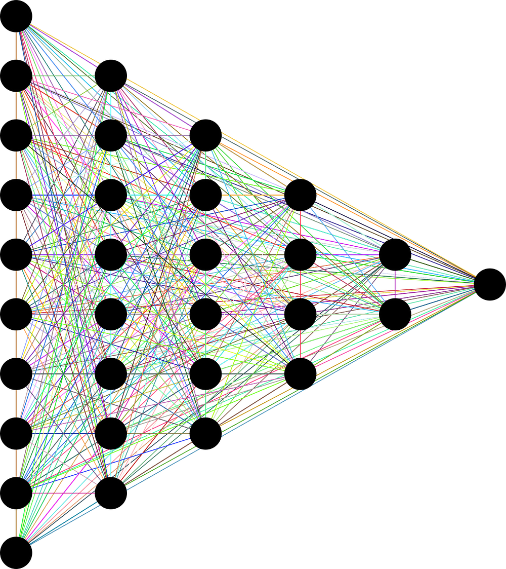
When a neural network is being trained, the first step is forward propagation. During the first epoch of training, random weights are considered (according to user-defined initializations) and are used to compute the required output values. At the end of the forward propagation, we receive some values at the output nodes.

With these received (or predicted) values, we compute the loss, which can be calculated as the difference between the predicted and actual values. Once the loss is calculated, it is time to adjust the weights of neural networks by differentiation and computation of gradients through the process of backpropagation.

In TensorFlow, the concept of automatic differentiation of gradients is used. This feature is of great importance as it helps in performing successful implementations of the backpropagation algorithm for training.

To differentiate automatically, TensorFlow needs to remember what operations happen in what order during the forward pass. Then, during the backward pass, TensorFlow traverses this list of operations in reverse order to compute gradients. We will understand the topic of Gradient Tape better in the coding section of this article, where we will implement a Gradient Tape function for performing automatic differentiation during the training procedure of the neural networks.

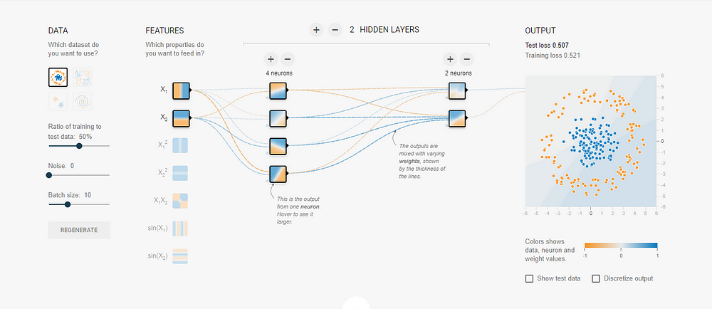
Before concluding this part, I would highly recommend the viewers who are beginner machine learning enthusiasts to check out the TensorFlow Playground website. It's a free website that allows you to visualize how neural networks perform on different datasets. It offers you a wide variety of options to try out and experiment with, while gaining a stronger intuition about how neural networks solve certain patterns and problems.

The next two sections of this article will only be briefly touched upon. Graphs, layers, and models will be covered in further detail in the next article as they are easier to work with when using the Keras module. The TensorFlow implementation of these concepts can be pretty confusing. Hence, these topics will only be touched briefly in this article.

Graphs

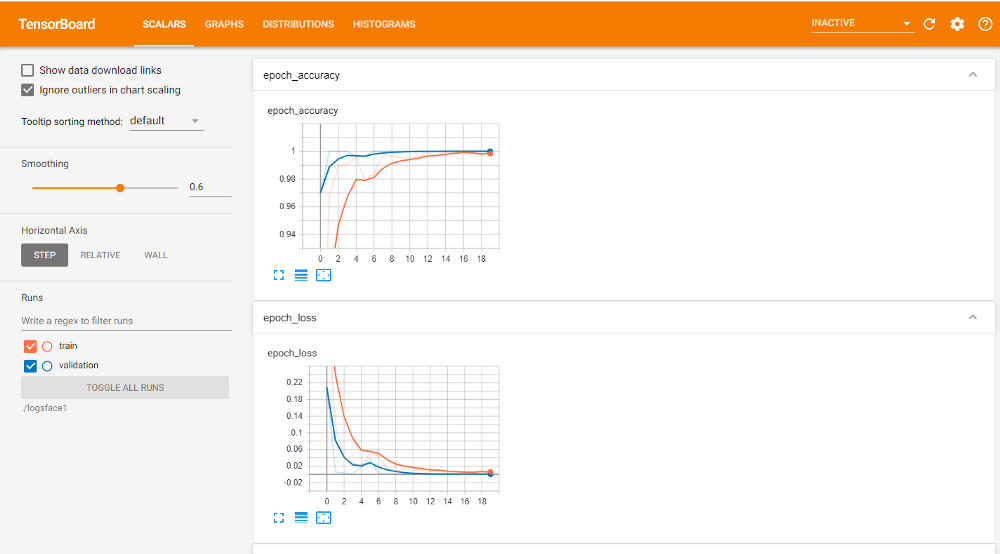
The concept of graphs in TensorFlow goes deeper than just a discussion of TensorFlow and Keras. The TensorBoard callback function available with the Keras module is definitely the better way to understand graphs and view your model performance.

However, to quickly gain a decent understanding of the topic of graphs in TensorFlow, Graphs are viewed as data structures that contain a set of tf.Operation objects, which represent units of computation. These tf.Tensor objects are a representation of the units of data that flow between various operations. These can be defined in a tf.Graph context. The best part about using these graphs is that they are data structures. They can therefore be saved, run, and restored, all without the original Python code.

Graphs are extremely helpful in analyzing models and seeing if a particular model is underfitting or overfitting the training data. Graphs help to understand the structure of the program and the required improvements to be made for higher performance. The topic of graphs will be covered in further detail in the next part of this series with TensorBoard.

Quick Introduction to Layers and Models

The topic of layers and models will be discussed in more detail in the next part of the series as well, because they are easier to build using the Keras library. However, in this section of the article, we will quickly focus on some essential aspects of TensorFlow for the construction of layers and models.

The TensorFlow library can be used to build your own custom models from scratch. Layers are functions with a known mathematical structure that can be reused, and have trainable variables. Multiple layers combined together and built for a single purpose can be used to create a model. We will discuss this topic further in the next part of the series. Let us now move on to understanding some simple but useful code in TensorFlow for basic purposes.

Understanding TensorFlow 2 With Code

In this final section of the article, we will explore some basic coding structures, patterns, and architectures that are required for programming high-level TensorFlow workflows for precise calculations and automatic computation of differentiation of gradients. We will mainly look at three areas for a better understanding of the TensorFlow library, namely, Gradient Clipping, Gradient Reversal, and Gradient Tape. The code provided here is just for reference, in order to gain a better and more intuitive understanding I highly recommend that you try writing it for yourself.

Gradient Clipping

In some neural network architectures (like Recurrent Neural Networks, or RNNs), there is often an issue of exploding and vanishing gradients that causes several errors and malfunctioning of the deep learning model built. To avoid and address this specific issue, the TensorFlow operation of Gradient Clipping can be performed to limit the values of the gradients to a specific range. Let us look at the following code block to understand this better.

@tf.custom_gradient
def grad_clip(x):
    y = tf.identity(x)
    def custom_grad(dy):
        return tf.clip_by_value(dy, clip_value_min=0, clip_value_max=0.5)
    return y, custom_grad

class Clip(tf.keras.layers.Layer):
    def __init__(self):
        super().__init__()
        
    def call(self, x):
        return grad_clip(x)
        

The above code block utilizes the custom_gradient function to develop gradient clipping that limits the values to a range bounded by a minimum and maximum value. Additionally, the class Clip can be used as a layer that can be added to clip the gradients of a specific hidden layer.

Gradient Reversal

The process of Gradient Reversal, as the name suggests, is used to reverse the gradients during the time of computation of a particular layer or sequence. The code block shown below is a simple representation of how such a gradient reversal can be performed, and how exactly it can be utilized in a custom layer for the purpose of reversing the gradients.

@tf.custom_gradient
def grad_reverse(x):
    y = tf.identity(x)
    
    def custom_grad(dy):
        return -dy   
    
    return y, custom_grad

class GradReverse(tf.keras.layers.Layer):
    def __init__(self):
        super().__init__()
        
    def call(self, x):
        return grad_reverse(x)
        

Gradient Tape

We have already discussed that backpropagation is one of the most essential concepts of deep learning and neural networks. The process of automatic differentiation to compute the gradients is extremely useful, and TensorFlow provides this in the form of the tf.GradientTape function. During eager execution, use tf.GradientTape to trace operations for computing gradients later.

tf.GradientTape is especially useful for complicated training loops. Since different operations can occur during each call, all forward-pass operations get recorded to a “tape”. To compute the gradient, play the tape backward and then discard. A particular tf.GradientTape can only compute one gradient; subsequent calls throw a runtime error.

def step(real_x, real_y):
    with tf.GradientTape() as tape:
        # Make prediction
        pred_y = model(real_x.reshape((-1, 28, 28, 1)))
        # Calculate loss
        model_loss = tf.keras.losses.categorical_crossentropy(real_y, pred_y)
    
    # Calculate gradients
    model_gradients = tape.gradient(model_loss, model.trainable_variables)
    
    # Update model
    optimizer.apply_gradients(zip(model_gradients, model.trainable_variables))
    

With this understanding of the Gradient Tape function, we have reached the end of the first part of the TensorFlow and Keras Series.

Conclusion

In this article, we have understood a brief history of the TensorFlow and Keras deep learning libraries. Then, we proceeded to learn about the different types of accelerators that are useful for neural network computations with a quick-starter guide. After this, we explored the various options that are available to data science enthusiasts to start building a wide variety of unique models and projects.

In the final two sections of this article, we looked at useful commands and guidelines to develop a deeper understanding of TensorFlow. We touched on essential topics like tensors, shape manipulation, constants and variables, backpropagation, and more. Finally, we ended the first part of the series with high-level TensorFlow code, which proves to be extremely useful for specific scenarios in deep learning and neural networks.

For further reading, I recommend you check out the official documentation of the TensorFlow Guide.

In the next part of this series, we will learn more about Keras and how the integration of Keras has positively affected the second version of TensorFlow. We will gain an intuitive understanding of the various layer options available in the Keras module, and learn how to utilize them to construct unique models from scratch to solve many different types of problems. We will also analyze the numerous callback options that we have available in Keras, and how you can create your own custom callbacks. Finally, we'll understand the compilation procedure and run-time training of deep learning models.

Until then, enjoy practicing!