The Absolute Guide to Keras

In this article, we will dive deeper into the world of TensorFlow and Keras. If you haven't already, I would highly recommend first checking out my previous article, The Absolute Guide to TensorFlow. It will help you to better understand the various concepts that we will cover in this article.

To quickly recap, so far we've discussed several aspects of TensorFlow, including how accelerators help to speed up computations; tensors, constants, and variables; backpropagation, graphs, layers, models, etc. Before we dive into the fundamentals and numerous essential aspects of Keras, let us take a quick look at the table of contents. Feel free to move forward to the sections that you find are the most relevant to you.

Table of Contents

• Introduction to Keras
• Learning Basic Layers
  1. Input Layer
  2. Convolutional and Max Pooling Layer
  3. Batch Normalization Layer
  4. Dropout Layer
  5. Dense Layer
• Understanding Various Model Architectures
  1. Sequential Models
  2. Functional API Models
  3. Custom Models
• Callbacks
  1. Early Stopping
  2. Checkpoint
  3. Reduce LR on Plateau
  4. TensorBoard
• Compilation and Training
• Conclusion

You can follow along with all of the code in this article and run it on a free GPU on a Gradient Community Notebook.

Introduction to Keras

TensorFlow is a deep learning framework used to develop neural networks. As we saw in the previous article, TensorFlow is actually a low-level language, and the overall complexity of implementation is high, especially for beginners. The solution to this issue is the introduction of another deep learning library that will simplify most of the complexities of TensorFlow.

The Keras deep learning library provides a more high-level approach to constructing neural networks. As described on their official website, Keras is an API that is designed for human beings, not for machines. This means that the module makes it simpler for humans to perform their coding operations.

The best part about using a deep learning library like Keras is that your work is significantly reduced, as you can build complex architectures within minutes while the module takes into account the actual procedure. Your focus remains on the overall architectural design, not the intricate details. Hence, Keras can be used as a more simplistic approach for users of all levels to attain the best performances. It also has a wide array of helpful documentation to get started. But, in this article, we will cover every single essential aspect about Keras that you need to know. So, without further ado, let us get started.

Learning Basic Layers

The Keras module enables users to construct neural networks with building blocks of elements called "layers". Each layer has its own specific function and operation. In this article, we will focus on gaining a better perception of how to use these layers without going into too much detail about how they work.

Let's look into a few basic layers, namely the input layer, convolutional and max-pooling layers, batch normalization layer, dropout layer, and dense layers. Although you can use the activation layer for activation functions, I usually prefer using them within other layers. We will discuss more about activation functions in the next section while constructing different architectures. For now, let us look into some of the basic layers that are used for building neural networks.

Input Layer

from tensorflow.keras.layers import Input

input1 = Input(shape = (28,28,1))

The input layer is one of the most basic layers which is usually used to define the input parameters of your model. As we will observe in the next section, we can usually skip the input layer in Sequential model implementation. However, it is required for some functional API models.

Convolutional and Max Pooling Layers (2-D)

from tensorflow.keras.layers import Convolution2D, MaxPooling2D

Convolution2D(512, kernel_size=(3,3), activation='relu', padding="same")
MaxPooling2D((2,2), strides=(2,2))

Convolutional layers create a convolution kernel that is convolved with the layer input to produce a tensor of outputs. The max-pooling layer is used to downsample the spatial dimensions of the convolutional layers, mainly to create location invariance while operating on images. We will discuss these layers in further detail in future articles when we work with computer vision tasks.

Batch Normalization Layer

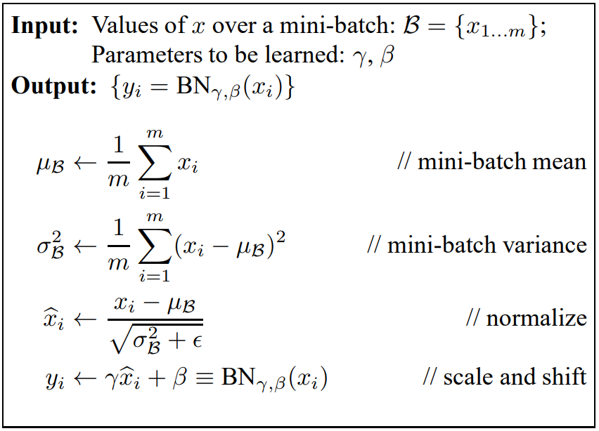
The above image is a representation of the implementation of the Batch Normalization layer from scratch. The role of this layer is to normalize the inputs by applying a transformation that maintains the mean output close to $0$ and the output standard deviation close to $1$. During the training stage, each batch of inputs has a separate calculation, and the normalization is performed accordingly. However, during the prediction stages (i.e., during test time), the values of the mean output and standard deviation are averaged for each batch.

Dropout Layer

These layers are often used to prevent model overfitting. Dropout layers will randomly drop a selected portion from the hidden nodes at the set rate, and train on the remaining nodes. When testing we don't drop any layers.

Dense Layer

These are the regular fully-connected layers that can be utilized for hidden nodes or the output layer for receiving a final prediction from the model built. These are the most basic building blocks of neural networks.

Understanding Various Model Architectures

Now that we have an intuition about the layers offered by Keras, let's also try to understand the various model architectures that we can use Keras to construct. Before we learn the different types of model architectures, we must first know what they are used for.

As a high-level library, Keras offers mainly three types of model architectures to work with that can be expanded with more layers and modules. These three model architectures include Sequential models, Functional API models, and Custom models (also called model subclassing). Each of these architectures has its own specific use cases, advantages, and limitations. Let's learn more about each of these model architectures individually, starting with the Sequential models.

Note: We will also briefly discuss more about the other layers that we have not covered in the previous section. We will then look at the concept of activation functions, learning a few activation functions and then proceeding to understand why and when they should be used.

Sequential Models

Sequential models are one of the simplest classes of model architectures offered by Keras. Once you import the Sequential class, you can use it to stack the numerous layers that we discussed in the previous section. The Sequential model is composed of a stack of layers, where each layer has exactly one input tensor and one output tensor.

The Sequential model architecture can be built in two separate ways. We will demonstrate both of these methods in the code below, where we build the same model architecture using both methods. We'll also look at the model summary to gain a better overall understanding of how these Sequential models work. Let's get started with the first method of constructing a model using the Sequential class of the Keras library.

Method I

from tensorflow.keras.layers import Convolution2D, Flatten, Dense 
from tensorflow.keras.layers import Dropout, MaxPooling2D
from tensorflow.keras.models import Sequential

model = Sequential()
model.add(Convolution2D(512, kernel_size=(3,3), activation='relu', padding="same", input_shape=(28, 28, 1)))
model.add(MaxPooling2D((2,2), strides=(2,2)))
model.add(Flatten())
model.add(Dense(10, activation='relu'))
model.add(Dropout(0.5))

To briefly explain the code, we can see that we imported all the required layers from the layers class. The above method is my preferred method of importing the layers, but you could also import the layers class from the module and build your model by calling the specific function and layer you want to construct. An example of this is as follows:

from tensorflow.keras import layers

layers.Convolution2D()
# Or:
layers.Dense()

We use the add function to stack layers on top of each other. We first stacked the convolutional layer with a specified input size, and then add a max-pooling operation to downsample the convolutional layer. Then, we added the flatten layer to condense all the material we have. Since we haven't already discussed the flatten layer, let's learn a bit more about it.

The flatten layer takes in an input and collapses the spatial dimensions of the input into a single value. However, it does not affect the batch size in any way. The main purpose of the flatten layer is to reduce the complex dimensionalities from the convolutional layers before passing it through a fully-connected neural network for computational operations.

After the flatten layer, we made use of the Dense layer to create a fully-connected neural network architecture. Finally, we used the Dropout layer to prevent overfitting. We have not yet added a final layer that would determine how our final output would look like; this is because I want to first cover more about activation functions.

The term "activation function" is derived from biological terms describing the synaptic activity of real neurons as they transfer information. In artificial neural networks, the activation function defines the output of a node given an input or set of inputs. The complete concept of activation functions is quite large, so for the purposes of this article we will briefly cover specific activation functions that you should know about.

The rectified linear unit (ReLU) activation function is one of the most popular activation functions, and is usually used by default in most neural network layers. This activation function helps prevent issues of exploding or vanishing gradients. Leaky ReLU is an alternate choice that performs better in specific scenarios. While we have other activation functions as well, let's now focus on the best activation functions to use for the final Dense layer of your model architecture.

If you have one node in the Dense layer, you can choose the linear activation function. When you have two nodes, a sigmoid activation function can be added. Finally, for multi-class problems we make use of the softmax activation function. In this case each label has a specific probability, where the class with the highest assigned probability is chosen. Equiped with this basic understanding of the different activation functions, let's proceed to look at the second method of construction of Sequential models with Keras.

Method II

from tensorflow.keras.layers import Convolution2D, Flatten, Dense
from tensorflow.keras.layers import Dropout, MaxPooling2D
from tensorflow.keras.models import Sequential

model1 = Sequential([
    Convolution2D(512, kernel_size=(3,3), activation='relu', padding="same", input_shape=(28, 28, 1)),
    MaxPooling2D((2,2), strides=(2,2)),
    Flatten(),
    Dense(10, activation='relu'),
    Dropout(0.5)
])

This pretty self-explanatory. The Sequential constructor is used with the desired layers specified.

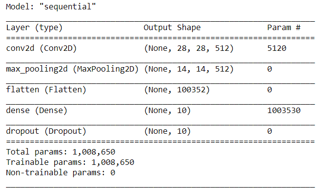
Let us now view the summary of both of these methods. The screenshot provided below is a representation of the layers, their output shapes, and the number of parameters.

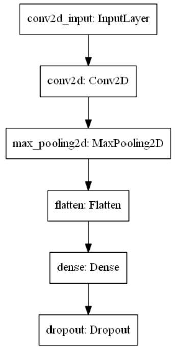
Let's us also have a brief look at the pictoral representation of the architecture we just built. The code below will save a model to your system, where you can view an image representing the numerous layers in your construction. Note that if you are trying to run the following code block locally on your system, you might also require additional installations like Graphviz.

from tensorflow import keras
from keras.utils.vis_utils import plot_model

keras.utils.plot_model(model, to_file='model.png', show_layer_names=True)

The above model summary is nearly the exact same for both methods of construction. You can verify the code on your respective system. Print the summaries for both architectures and review the model type–which is sequential in both cases–and review the placements of layers, their output shapes, and finally, their parameters. Sequential models are the most straightforward way to create neural networks, but they may always not be the best choice. Let's find out why while considering the next model architecture.

Functional API Models

While Sequential models are simple to construct, they may not be the best choice in several scenarios. When you have a nonlinear topology or require a branch-like architecture, then the appropriate models cannot be constructed with the Sequential architecture. The image below summarizes when Sequential models should not be used.

For such cases we use functional API models, which offer great flexibility and allow you to build non-linear topologies. Functional API models support shared layers and multiple inputs and outputs. Let's look at a simple code block to construct a similar architecture as what we did with the Sequential models.

Code

from tensorflow.keras.layers import Convolution2D, Flatten, Dense, Dropout
from tensorflow.keras.layers import Input, MaxPooling2D
from tensorflow.keras.models import Model


input1 = Input(shape = (28,28,1))
Conv1 = Convolution2D(512, kernel_size=(3,3), activation='relu', padding="same")(input1)
Maxpool1 = MaxPooling2D((2,2), strides=(2,2))(Conv1)
Flatten1 = Flatten()(Maxpool1)
Dense1 = Dense(10, activation='relu')(Flatten1)
Dropout1 = Dropout(0.5)(Dense1)
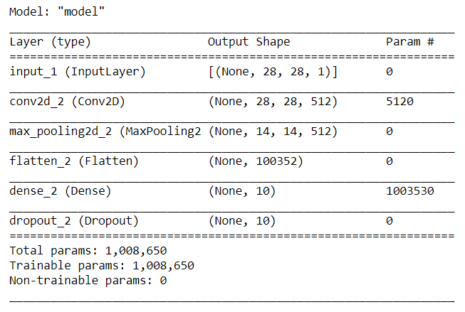
model = Model(input1, Dropout1)

The model summary is as follows.

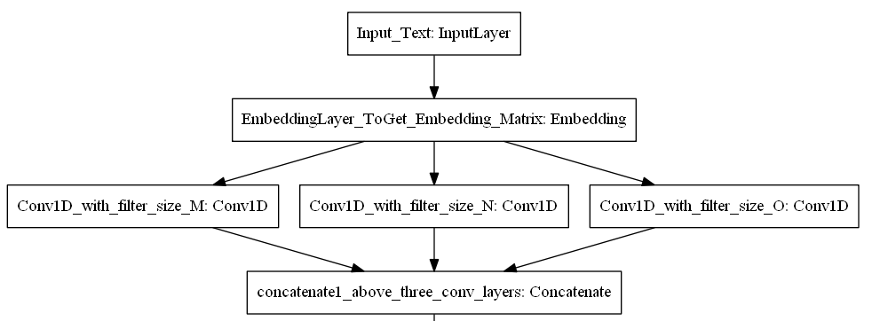
And the model plot is as follows.

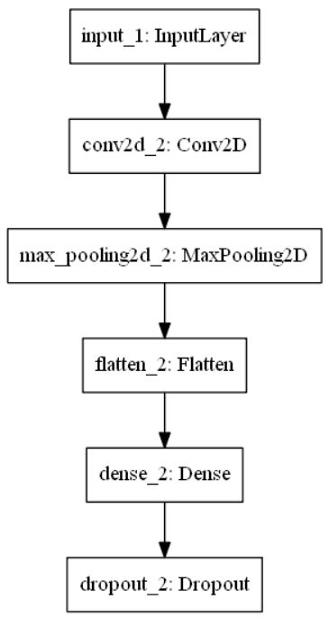
With the model summary and plotting, we can determine that the functional API can be used for constructing models similar to Sequential architectures as well as those with unique nonlinear topologies. Hence, functional API models have diverse use cases and are consistently used among developers for creating complex neural network architectures.

Custom Models

Custom models (or model subclassing) is where you implement the entire neural network architecture from scratch. While the functional API offer is highly flexible and is used most commonly by developers, sometimes custom models are used for specific research purposes. You construct your own architectures from scratch and have complete control over their functioning. A code block for the implementation of one such use case from one of my projects is shown below.

import tensorflow as tf

class Encoder(tf.keras.Model):
    '''
    Encoder model -- That takes a input sequence and returns output sequence
    '''

    def __init__(self, inp_vocab_size, embedding_size, lstm_size, input_length):
        super(Encoder, self).__init__()
        
        # Initialize Embedding layer
        # Intialize Encoder LSTM layer
        
        self.lstm_size = lstm_size
        self.embedding = tf.keras.layers.Embedding(inp_vocab_size, embedding_size)
        self.lstm = tf.keras.layers.LSTM(lstm_size, return_sequences=True, return_state=True)

    def call(self, input_sequence, states):
        
        '''
          This function takes a sequence input and the initial states of the encoder.
          Pass the input_sequence input to the Embedding layer, Pass the embedding layer ouput to encoder_lstm
          returns -- All encoder_outputs, last time steps hidden and cell state
        '''
        
        embed = self.embedding(input_sequence)
        output, state_h, state_c = self.lstm(embed, initial_state=states)

        return output, state_h, state_c
    
    def initialize_states(self,batch_size):
        
        '''
        Given a batch size it will return intial hidden state and intial cell state.
        If batch size is 32- Hidden state shape is [32,lstm_units], cell state shape is [32,lstm_units]
        '''
    
        return (tf.zeros([batch_size, self.lstm_size]),
                tf.zeros([batch_size, self.lstm_size]))
              

With these three main architectures taken into consideration, you can freely construct your deep learning models to accomplish specific projects or tasks. That being said, the journey of the deep learning model is not yet fully completed.

We will learn more about callbacks in the next section. Finally, we will learn about model compilation and training stages.

Callbacks

Callbacks play a significant role in model training. A callback is an object that can perform actions at various stages of training, such as at the start, middle, or end of an epoch. It can also affect training at the start or end of a batch.

Although there are a lot of callbacks availble in Keras, we will focus on only a few of the most essential ones that are usually used while constructing deep learning models. During the training (or "fitting") stages of the model, the most commonly used callbacks are early stopping, checkpoint, reduce LR on plateau, and TensorBoard. We will briefly consider each of these callbacks with their respective code.

Early Stopping

from tensorflow.keras.callbacks import EarlyStopping

early_stopping_monitor = EarlyStopping(patience=2)

When the early stopping callback finds that there is no significant improvement compared to previous epochs of training, the training procedure is stopped after the specified patience. In this case, after any two epochs, if the validation loss does not improve, the training procedure is stopped.

Model Checkpoint

from tensorflow.keras.callbacks import ModelCheckpoint

checkpoint = ModelCheckpoint("checkpoint1.h5", monitor='accuracy', verbose=1,
                              save_best_only=True, mode='auto')

The Model Checkpoint callback in Keras saves the best weights achieved during the training process. While training, there is a chance your model starts to underperform after some epochs, either due to overfitting or other factors. Either way, you always want to ensure that the best weights are saved for performance on your tasks.

You can store the checkpoint with a name of your choice. It is usually preferable to monitor the best validation loss (using val_loss), but you can alternatively choose to monitor any of your preferred metrics. The main benefit of using ModelCheckpoint is storing the best weights of your model so that you can use them later for testing or deployment purposes. By saving the stored weights, you can also restart the training procedure from that point.

Reduce LR On Plateau

from tensorflow.keras.callbacks import ReduceLROnPlateau

reduce = ReduceLROnPlateau(monitor='accuracy', factor=0.2, patience=10, 
                           min_lr=0.0001, verbose = 1)

While fitting the model, after a certain point, the model may stop improving. At this point it is often a good idea to reduce the learning rate. The factor determines the rate at which the initial learning rate must be reduced, which is new_lr = lr * factor.

After waiting the specified number of epochs (the patience, in this case, 10), if there are no improvements, then the learning rate is reduced by the stated factor. This reduction continues to take place until the minimum learning rate is reached.

Callbacks work independently. Hence, if you are using a patience of 10 for ReduceLROnPlateau, it is a good idea to increase your EarlyStopping callback patience as well.

TensorBoard

from tensorflow.keras.callbacks import TensorBoard

logdir='logs'
tensorboard_Visualization = TensorBoard(log_dir=logdir)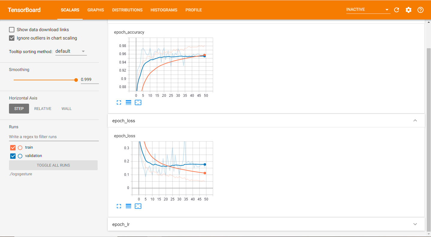

The TensorBoard callback is one of the most valuable tools available to users. With it, you are able to graphically visualize your training procedure and easily discover trends in the working of your models. For instance, from your analysis you can determine after how many epochs model training can be stopped, and which epoch achieves the best results. Apart from this, it provides developers many options to analyze and make improvements to their models.

Another essential aspect of Keras is that it provides the ability to create your own custom callbacks for specific use cases. We will discuss more on this topic in future articles as we use them. However, if you are interested in learning more about creating your own custom callback functions, feel free to visit the following website.

Compilation and Training

The next stage after building your model architecture and defining your callbacks is to implement the model compilation and training steps. Thankfully, with the help of Keras both of these steps are incredibly simple and involve little code.

Model Compilation

model.compile(loss='categorical_crossentropy',
              optimizer = Adam(lr = 0.001),
              metrics=['accuracy'])

The compilation process in Keras configures the model for the training procedure. In this step, you define some of the most essential parameters, such as the loss function, optimizer, and the metrics apart from "loss" that you want to track while training the model. The loss function used will vary from one problem to another, while the optimizer will usually be the Adam optimizer. Other options (like RMSprop) can be tried out as well to see what suits your model best. Once you have finished compiling the model, you can proceed to model training.

Fitting the Model

model.fit(train_generator,
          steps_per_epoch = train_samples//batch_size,
          epochs = epochs,
          callbacks = [checkpoint, reduce, tensorboard_Visualization],
          validation_data = validation_generator,
          validation_steps = validation_samples//batch_size,
          shuffle=True)

Once we finish compiling the model, we can fit the model on the training dataset. The fit function trains the model for a fixed number of epochs (iterations on a dataset). For a better understanding of how steps like backpropagation work, I would highly recommend checking out the first part of this series. The basic parameters you need to define are the training data, number of epochs, batch size, and callbacks.

Finally, we use model.evaluate() to evaluate the overall performance of the model. This function is useful to measure how well the model performs, and if it's ready for deployment. Then, we can make use of the model.predict() function to make predictions on new data.

Conclusion

In this article, we covered the second part of our Absolute Guide to TensorFlow and Keras. In the introduction we saw that Keras is a high-level API that offers an alternate simplistic approach to the complex coding requirements of TensorFlow. We then gained an intuition regarding some of the layers which can be constructed with the help of the Keras library.

With a basic intuition behind some of the layers in the Keras module, it becomes easier to understand the various model architectures that can be constructed. These architectes include Sequential models, Functional API models, and Custom models. Depending on the complexity of your particular task, you can decide which option suits your project best. We also briefly covered the utility of activation functions and their usage.

From there we moved on to understand the significance of callback functions that are offered by Keras. Apart from learning some of the essential callbacks, we also focused on the TensorBoard callback that you use to analyze the performance of your models at regular intervals.

Finally, we covered compilation and training procedures. Once the models are built, you can save them and even deploy them for a wide range of audiences to benefit from them.

This two-part series on TensorFlow and Keras should give you a fundamental understanding of the utility of these libraries, and how you can use them to create amazing deep learning projects. In an upcoming article, we will learn another essential deep learning concept: transfer learning, with lots of examples and code. Until then, enjoy your coding!