In Part One, we covered the basic components of GauGAN as well as the loss functions it makes use of. In this part, we'll cover the training details and see how to set up training on your own custom dataset.
Part One is necessary for understanding how the training process works, but if you're not interested in the training details and just want to implement GauGAN on your own data, feel free to skip directly to the section titled Custom Training. In Part 3 we'll cover model evaluation techniques, and we'll close this series by looking at how to debug training and deciding if GauGAN is right for you.
You can also follow along with the code in this tutorial on the ML Showcase, and run the model on a free GPU.
Before we start, another important thing to note is that the open-source implementation by Nvidia differs in many ways from what is reported in the official paper. This is understandable, considering almost a year has passed since it was published. I will do my best to point out these differences whenever possible.
Launch Project For Free
Training Details
Pre-processing Steps
GauGAN is trained with images of only one size and aspect ratio. This means that once trained, GauGAN is only guaranteed to work best with images of the same size as what it was been trained on. If the image used during inference is either too small or too large, expect the output to considerably degrade.
There are various methods which can be used to resize or crop the image to the size required by GauGAN.
Weight Initialization
The authors report use of Glorot initialization, whereas this implementation uses the default PyTorch initialization for convolutional layers which is the Kaiming Uniform Initialisation.
Learning Rate Policy
The number of epochs trained will of course depend on the dataset being used and the complexity of the type of data one is training on. The default learning rate is set to be 0.0002.
The implementation also makes use of Two Time-Scale Update Rule learning policy. In this, we chose different learning rates for the generator and the discriminator. Generally, the generator's learning rate is kept lower than the discriminator so as to allow the generator to perform better by learning slowly, leading to more stabilised learning.
For the first half of the total number of epochs, the training learning rate option lr is kept constant to the value it's initialised with. Both the discriminator as well as the generator are trained with this learning rate.
In the second half, the learning rate option lr is decayed linearly to zero, being updated each epoch. For each update, the discriminator learning rate is set lr * 2 whereas the generator learning rate is set to lr / 2.
Batch Size
The batch size generally depends upon how large an image you are trying to synthesise. GauGAN may require a lot of GPU resources to work well. Training the default GauGAN as provided in the implementation on images of size 768 x 576 with batch size of 1 takes about 12 GB of GPU memory. The ReadMe file from Nvidia's open sourced implementation reads:
To reproduce the results reported in the paper, you would need an NVIDIA DGX1 machine with 8 V100 GPUs
This equals 128 GB of memory. Yikes!
Optimizer
Adam optimizer is used for the generator as well as the discriminator. $\beta_1$ and $\beta_2$ are set to 0.5 and 0.999 respectively.
Custom Training
Test Run
In this part, we look at how to set up training using a custom dataset. We begin by getting GauGAN from GitHub and installing all of the necessary dependencies.
git clone https://github.com/NVlabs/SPADE.git
cd SPADE/
pip install -r requirements.txt
If you do not have pip, you can manually look up the packages in the file requirements.txt and install them through conda.
Then, you must install synchronized batch norm.
cd models/networks/
git clone https://github.com/vacancy/Synchronized-BatchNorm-PyTorch
cp -rf Synchronized-BatchNorm-PyTorch/sync_batchnorm .
cd ../../
Once this is done, let us give it a test run. Start by grabbing the pre-trained models. Currently Nvidia provides pre-trained models for COCO-stuff, Cityscapes and the ADE20K datasets.
First, download the models from this google drive link. Create a folder named checkpoints and place the downloaded file inside the folder. Then unzip it.
cd checkpoints
tar xvf checkpoints.tar.gz
cd ../
Now you can run the model for either of the three datasets, but let's run the one for COCO-stuff. Because the github repo we just cloned already has some sample files from the COCO stuff dataset, this will save us some time.
Make sure you are inside the SPADE folder and run:
python test.py --name coco_pretrained --dataset_mode coco --dataroot datasets/coco_stuff
Now, if you are using PyTorch version > 1.1, the code might throw up the following error and may stop.
Traceback (most recent call last):
  File "test.py", line 36, in <module>
    generated = model(data_i, mode='inference')
  File "/home/ayoosh/miniconda3/lib/python3.7/site-packages/torch/nn/modules/module.py", line 541, in __call__
    result = self.forward(*input, **kwargs)
  File "/home/ayoosh/work/SPADE/models/pix2pix_model.py", line 43, in forward
    input_semantics, real_image = self.preprocess_input(data)
  File "/home/ayoosh/work/SPADE/models/pix2pix_model.py", line 130, in preprocess_input
    instance_edge_map = self.get_edges(inst_map)
  File "/home/ayoosh/work/SPADE/models/pix2pix_model.py", line 243, in get_edges
    edge[:, :, :, 1:] = edge[:, :, :, 1:] | (t[:, :, :, 1:] != t[:, :, :, :-1])
RuntimeError: Expected object of scalar type Byte but got scalar type Bool for argument #2 'other' in call to _th_or
This happens because of introduction of the bool datatype in PyTorch 1.1+. The simple solution is to go to the function get_edges in the file models/pix2pix_model.py and make a simple change.
Add the line edge = edge.bool after the first line of the function. All in all, your function get_edges should look like this:
def get_edges(self, t):
    edge = self.ByteTensor(t.size()).zero_()
    edge = edge.bool()
    edge[:, :, :, 1:] = edge[:, :, :, 1:] | (t[:, :, :, 1:] != t[:, :, :, :-1])
    edge[:, :, :, :-1] = edge[:, :, :, :-1] | (t[:, :, :, 1:] != t[:, :, :, :-1])
    edge[:, :, 1:, :] = edge[:, :, 1:, :] | (t[:, :, 1:, :] != t[:, :, :-1, :])
    edge[:, :, :-1, :] = edge[:, :, :-1, :] | (t[:, :, 1:, :] != t[:, :, :-1, :])
    return edge.float()
Now, your code should run and you can find the results by opening the file results/coco_pretrained/test_latest/index.html in your browser.
Setting Up Your Data
You will first need to set up your training data in a way that can be read by GauGAN's implementation.
Essentially, you will need semantic segmentation maps, as well as their corresponding real images to get started. Optionally, you can also use instance segmentation maps, which might boost your performance.
For demonstration purposes, we use the CamVid dataset. Let's start by creating the folder to store the datasets.
mkdir -p datasets/CamVid
cd datasets/CamVid
Then we download the dataset.
wget -c http://web4.cs.ucl.ac.uk/staff/g.brostow/MotionSegRecData/files/701_StillsRaw_full.zip
unzip 701_StillsRaw_full.zip
Then, get the annotations.
wget -c http://web4.cs.ucl.ac.uk/staff/g.brostow/MotionSegRecData/data/LabeledApproved_full.zip
mkdir LabeledApproved_full
cd LabeledApproved_full
unzip ../LabeledApproved_full.zip
cd ..
GauGAN requires the semantic segmentation maps to be images with one channel, where each pixel represents the index of the semantic class it belongs to. If your semantic segmentation maps are in RGB or Polygon format, then you need to convert them to the mentioned format. You also need to make sure that the class indices are continuous integers from 0 to n-1 where n is the number of classes.
CamVid dataset has it's semantic segmentation maps in RGB format. Let us convert them to format required by GauGAN.
We first begin by creating a folder to store our new annotations. Assuming you are in the directory datasets/CamVid, run
mkdir GauGAN_Annotations Then, create a python script called convert_annotations.py in the CamVid folder.
touch convert_annotations.py
We will also be needing the list of colors corresponding to each label in the CamVid dataset.
wget http://mi.eng.cam.ac.uk/research/projects/VideoRec/CamVid/data/label_colors.txtPreparing Semantic Segmentation Maps
We will now populate the script convert_annotations.py with code to do the conversion. First import the necessary stuff.
import numpy as np
import os
import cv2
from copy import deepcopy
from tqdm import tqdm
Then, we write a function to extract the labels from the text file to a numpy array.
with open("label_colors.txt", "r") as file:
    label_colors = file.read().split("\n")[:-1]
    label_colors = [x.split("\t") for x in label_colors]
    colors = [x[0] for x in label_colors]
    colors = [x.split(" ") for x in colors]

for i,color in enumerate(colors):
    colors[i] = [int(x) for x in color]

colors = np.array(colors)
Get the addresses of the annotation files to work on.
annotations_dir = "LabeledApproved_full"
annotations_files = os.listdir(annotations_dir)
annotations_files = [os.path.join(os.path.realpath("."), annotations_dir, x) for x in annotations_files]
Now, we run through each of theses files in a loop. We then nest a loop inside this loop, which loops through each label class, checks which pixels belong to the label class (by checking RGB value) , and assigns them an class index.
for annotation in tqdm(annotations_files):
    # for each file
    img = cv2.imread(annotation)[:,:,::-1]

    h,w, _ = img.shape

    modified_annotation = np.zeros((h,w))

    for i,color in enumerate(colors):
    	# for each class color, i is the index value
        color = color.reshape(1,1,-1)
        mask = (color == img)

        r = mask[:,:,0]
        g = mask[:,:,1]
        b = mask[:,:,2]

        mask = np.logical_and(r,g)

        mask = np.logical_and(mask, b).astype(np.int64)

        mask *= i

        modified_annotation += mask

    save_path = annotation.replace(annotations_dir, "GauGAN_Annotations")
    cv2.imwrite(save_path, modified_annotation)
Check your GauGAN_annotations folder to see the converted SegMaps. You can get the entire script here
Preparing Instance Segmentation Maps
Using instance maps is optional. However, shall you use them, you need to convert them into images with one channel where each pixel belonging to each instance must have different values. Unlike semantic segmentation maps, instance indices not have to be integers in range 0 to n-1. Having a different, albeit, arbitrary integer for each instance will do.
This is because the code responsible for create edge maps (refer to the previous post to read about edge maps) only looks at difference between pixels. So it does not matter if three of your instances are encoded as {0,1,2} or {34, 45, 50}. You can also omit instances for background object and set the values to a background index, say,0.
Generally, any instance instance segmentation algorithm (like Mask RCNN) or annotation tool gives different IDs to each instance rather than colors so your job will be easier. For example, the convention Cityscapes follows is {class_index}000{instance_id}. For example, a couple of instances of a car would be labelled as 120001 and 120002 where 12 is the index for car class, and 1 and 2 are the instances of the car.
Instance IDs are useful when you have a lot of overlapping objects of the same class. In case there are no instances, I have tried using the semantic labels themselves as instances. It does not really work.
Partitioning Your Dataset
There are two ways to partition your dataset.
- Partition the dataset first, and run the preprocessing scripts on each partition separately.
- Do the partition after doing the preprocessing.
In our case, we do step 2. For sake of simplicity, I am only partitioning the data between train and test sets. You can carve out a validation set too.
First, let us create four folders to house our parts. Make sure you run this code from datasets/CamVid
mkdir train_img train_label test_img test_labelNote that if you are using instance maps as well, you will also need to create train_inst and test_inst as well.
Now, create a file that contains the partitioning code.
touch partition_data.py
Let us now write code for partitioning in this file. First, import the required libraries.
import os
from shutil import copy
import random
from tqdm import tqdm
Then, we create a list of files that belong to the training set and the test set.
partition_percentage = 90
annotations_dir = 'GauGAN_Annotations'
annotations_files = os.listdir(annotations_dir)
annotations_files = [os.path.join(os.path.realpath("."), annotations_dir, x) for x in annotations_files]

train_labels = random.sample(annotations_files, int(partition_percentage / 100 * len(annotations_files)))
test_labels   = [x for x in annotations_files if x not in train_labels]

train_images = [x.replace(annotations_dir, '701_StillsRaw_full').replace("_L", "") for x in train_labels]
test_images  = [x.replace(annotations_dir, '701_StillsRaw_full').replace("_L", "") for x in test_labels]
Here, we use a partition percentage of 80-20 percent for train-test split. Now, we copy the files to their respective folders we created above using python's shutil package.
for file in tqdm(train_labels):
    src = file
    dst = file.replace(annotations_dir, 'train_label').replace("_L", "")
    copy(src, dst)

for file in tqdm(test_labels):
    src = file
    dst = file.replace(annotations_dir, 'test_label').replace("_L", "")
    copy(src, dst)

for file in tqdm(train_images):
    src = file
    dst = file.replace('701_StillsRaw_full', 'train_img')
    copy(src, dst)

for file in tqdm(test_images):
    src = file
    dst = file.replace('701_StillsRaw_full', 'test_img')
    copy(src, dst)
You can get the entire script here
And we are done! Let's train the model now.
Training The Model
Before we run the training, let me go over some compatibility issues. The TensorBoard logging code doesn't work with TF 2.0, since the latest version has brought major changes to TensorBoard and Summary syntax. You will also need to make sure your version of scipy <= 1.2.0. You can also run into some issues if you are using PIL 7.0, so it may be better to use 6.1.0 instead.
pip install tensorflow==1.15.0
pip install scipy==1.2.0
pip install pillow==6.1.0
To train the model, we go to the main folder SPADE and run the following command.
python train.py --name CamVid --dataset_mode custom --no_instance --label_nc 32 --preprocess_mode scale_width --label_dir datasets/CamVid/train_label --image_dir datasets/CamVid/train_img/ --load_size 512 --aspect_ratio 1.3333 --crop_size 512 --ngf 48 --ndf 48 --batchSize 1 --niter 50 --niter_decay 50 --tf_log This will kick the training off. Let us understand what each parameter means.
nameWhatever name you give here, a folder will be the same name will be created incheckpointsdirectory (checkpoints/name). This folder will contained your saved weights, TensorBoard logs and intermediate training results. ( can be seen bycheckpoints/name/web/index.html)dataset_modeThis can be set to either COCO-Stuff, Cityscapes, ADE20K or custom. It's set to custom in our case. This mode allows us to define the image and labels directory for training usingimage_dirandlabel_dirflags.label_ncYou will need to set to the number of classes in your dataset, which is 32 in CamVid.preprocess_modeThis basically defines how are we going to resize our image to the size that is accepted by the network. I have chosenscale_widthwhich means that the width is scaled to the value defined by the parameterload_size, while keeping the aspect ratio same (meaning height changes). You could alternatively chose options like simplyresize( resizes non-isometrically to (loadsize,loadsize) ,crop(where the a portion of size (crop_size,crop_size) is cropped from the image) andnone(Which will resize both height and width to closest multiple of 32). These can be used in combination too. For example,scale_width_crop, which will scale the image's width toload_sizeand then make a crop ofcrop_size. The code governing this functionality can be found inget_transformfunction indata/base_dataset.py.aspect_ratiois basically the aspect ratio of the image. GauGAN's code is weird in the sense thatcrop_sizeis always used to finally resize the image, even if nocropoptions are used in in thepreprocessmethod. Therefore, you will have to setcrop_sizeregardless whether you are usingcropor not. This can be found out in in thecompute_latent_vector_sizemethod of classSPADEGeneratorin the filemodels/networks/generator.py`.
    def compute_latent_vector_size(self, opt):
        if opt.num_upsampling_layers == 'normal':
            num_up_layers = 5
        elif opt.num_upsampling_layers == 'more':
            num_up_layers = 6
        elif opt.num_upsampling_layers == 'most':
            num_up_layers = 7
        else:
            raise ValueError('opt.num_upsampling_layers [%s] not recognized' %
                             opt.num_upsampling_layers)


        sw = opt.crop_size // (2**num_up_layers)


        sh = round(sw / opt.aspect_ratio)

        return sw, sh
As you can see in line 16, the sh the height of input is computed by scaling the width to crop_size and keeping aspect ratio aspect_ratio. So, I have used load_size for loading the images and the same value for crop_size for the above operation. The above also means that your aspect ratio is fixed. You will have to hack around this piece of code to make it run on an arbitrary aspect ratio.
ngfandndf. Basically the convolutional filters in the first layer of the generator and discriminator respectively. The number of filters in subsequent layers is a function of these numbers. Therefore, these numbers are sort of a measure of capacity of your networks.batchSize. Well, the name is obvious. Ain't it?niterandniter_decay. Your learning rate will stay constant forniterepochs, and decay linearly to zero forniter_decayoptions. So technically, you train forniter + niter_decayepochs.tf_log. Using this makes the code log your losses and intermediate results in thecheckpoints/name/logs
Training Your Model on Multiple GPUs
If you have multiple GPUs, you can use multiple GPU training by using the gpu_ids flag.
python train.py --name CamVid --gpu_ids 0,1 --batch_size 2 --dataset_mode custom --no_instance --label_nc 32 --preprocess_mode scale_width --label_dir datasets/CamVid/train_label --image_dir datasets/CamVid/train_img/You need to make sure that the batch_size is a multiple of the number of GPUs you are going to use, otherwise, the code will throw up an error. This is because the batch needs to be divided across GPUs.
Resuming Training
If your training gets interrupted, you can resume it using --continue_training flag. Model checkpoints are updated after every fixed number of loop iterations defined by the flag --save_latest_freq. continue_train will resume training from the latest checkpoint.
In addition to the latest checkpoint, learned weights are stored every fixed number of epochs, the frequency being defined by --save_epoch_frequency. By default, this number is 10, and if you want to start from any of these epochs instead of the latest one, you can use a combination --continue_training --which_epoch 20 to resume training from, say, the 20th epoch.
Running Inference
Once your training is done, you can run inference with the following command.
python test.py --name CamVid --dataset_mode custom --no_instance --label_nc 32 --preprocess_mode scale_width --label_dir datasets/CamVid/test_label --image_dir datasets/CamVid/test_img/ --load_size 512 --aspect_ratio 1.3333 --crop_size 512 --ngf 48Notice how we have changed the data directories to test_img and test_label . The results will be saved in the results/CamVid/test_latest folder.
The CamVid dataset is severely lacking when it comes to diversity. Firstly, because it's too small. Secondly, because it's made up of frames from a video stream, meaning that many frames are going to be correlated. This is true especially for frames where the vehicle is stationary, meaning that the background will be stationary as well. For these reasons, even a good choice of parameters can lead to mediocre results.
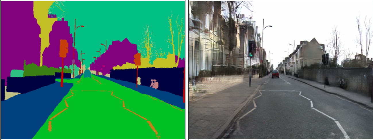
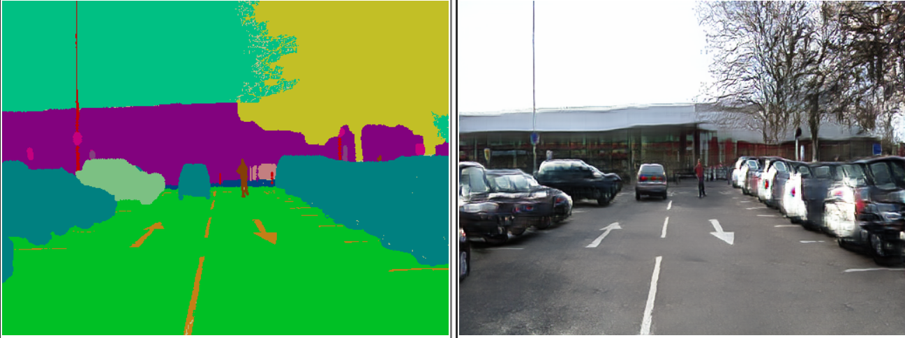
Let's have a look at some results, starting with decent predictions.
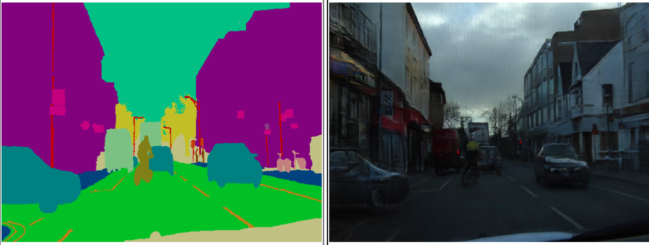
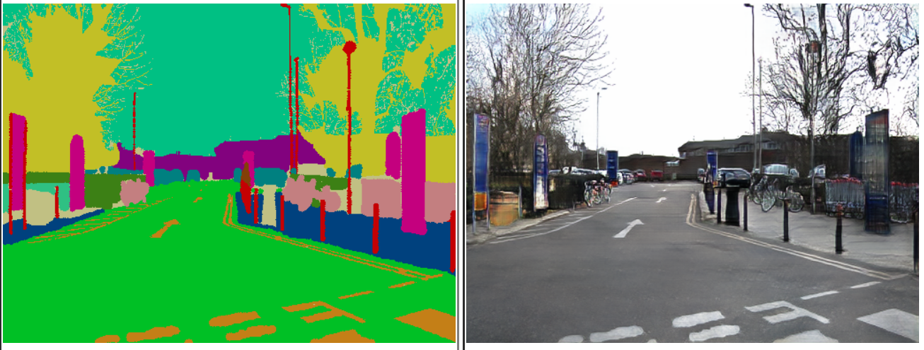
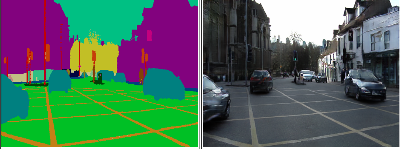
And here are some of the bad ones.
Whenever our vehicle stops at a signal, we tend to get a lot of similar frames due to the vehicle seeing the same thing again and again. This causes the network to overfit, especially when our dataset is so small.
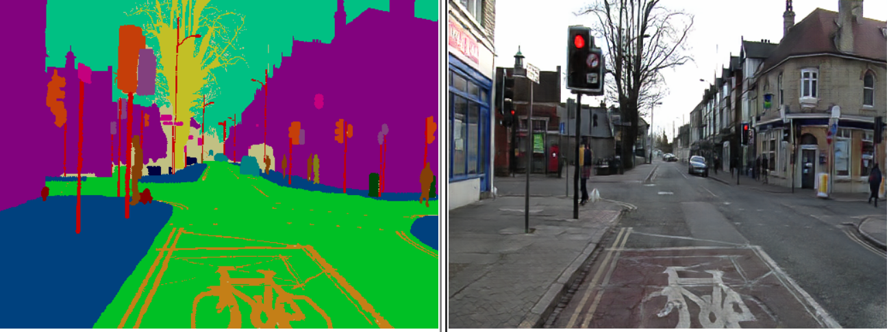
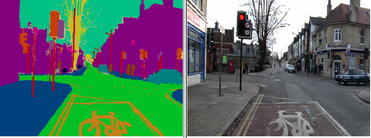
We see that the overfitting is so bad that the network has even memorized the color of the traffic light; it's always a red light.
Conclusion
In Parts 3 and 4, will talk more about considerations for our data when it comes to effectively training GauGAN, and why CamVid is a bad choice. In the next post in particular, we'll how well GauGAN performs compared to other similar algorithms, and how to use the FID score to evaluate its performance.
Understanding GauGAN Series
- Part 1: Unraveling Nvidia's Landscape Painting GANs
- Part 2: Training on Custom Datasets
- Part 3: Model Evaluation Techniques
- Part 4: Debugging Training & Deciding If GauGAN Is Right For You