Understanding GauGAN Part 1: Unraveling Nvidia's Landscape Painting GANs

One of the most interesting papers presented at CVPR in 2019 was Nvidia's Semantic Image Synthesis with Spatially-Adaptive Normalization. This features their new algorithm, GauGAN, which can effectively turn doodles into reality. The technology has been in the works for some time, starting from Nvidia's debut of Pix2PixHD in 2017 and Vid2Vid in 2018. Finally, 2019 gave us the impressive addition of GauGAN. It'll be interesting to see what Nvidia has in store for 2020.

In this article we'll see how the GauGAN algorithm works on a granular level. We'll also gain insight into why Nvidia is investing so heavily in the use of these algorithms.

I'd also like to point out that in this post I'll focus primarily on GauGAN, and avoid going too deep into Pix2PixHD in this post. Both of these algorithms generate images and have a lot in common, with GauGAN being a more recent development. I'll therefore focus on GauGAN and only mention Pix2PixHD when there is a feature which is strikingly different from GauGAN, mainly to avoid repetitiveness.

This is the first part in a four part series. We'll also cover:

• Training on Custom Datasets
• GauGAN Evaluation Techniques
• Debugging Training & Deciding If GauGAN Is Right For You

You can also check out GauGAN on the ML Showcase, and run the model on a free GPU.

Let's get started!

Conditional GANs

GANs are typically used to generate data. You typically provide a noisy input which the network will use to produce a related output. This type of GAN is useful in the sense that it doesn't need anything to generate data other than random noise, which can be generated using any numeric software.

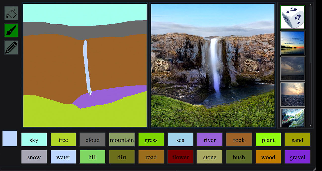
On the other hand, Conditional GANs generally take a specific input which determines the data to be generated (in other words, the generated data is conditioned upon the input we provide). For example, in GauGAN, the input is a semantic segmentation map and the GAN generates a real image conditioned upon the input image, like in the following example.

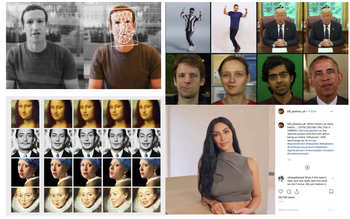
Similarly, other conditional generative networks might create:

1. A video frame conditioned on the previous frame.
2. A terrain map image conditioned on the plain map image.
3. An image conditioned on a text description.

And much more.

Architecture of GauGAN

Like any other generative adversarial network, GauGAN contains a discriminator and a generator. With GauGAN specifically, Nvidia has introduced a new normalization technique called Spatially Adaptive Normalization, or SPADE Normalization, via use of special SPADE blocks. Additionally, GauGAN features an encoder that is used for multi-modal synthesis (if this doesn't make sense, don't worry – we'll cover it later).

The input to the generator consists of:

1. A one-hot encoded semantic segmentation map
2. An edge map (optional)
3. An encoded feature vector (optional)

The first is necessary, whereas the second and third inputs are optional. Whichever set of inputs are used, they are depth-concatenated before being sent to the generator.

The semantic segmentation map is basically one-hot encoded such that we have a one-hot encoded map of each class. These maps are then depth-concatenated.

An edge map is only possible if one has instance IDs for objects in the image. In segmentation labels, we only care about the class of the object. If two cars are overlapping, then the car label would be a blob consisting of two overlapping cars. This might confuse the algorithm and cause it to perform worse when two objects are overlapping.

To overcome this, the utilization of a semantic label map was introduced in Pix2PixHD. This is a 0-1 binary map where every pixel is zero except those where each of the four neighbors do not belong to the same instance.

An encoded feature vector is produced by passing the image which will be used as the style guide through the encoder.

Generator

The generator of GauGAN is a fully convolutional decoder consisting of SPADE blocks. SPADE stands for Spatially Adaptive Normalization blocks. We will discuss this component in detail when we are done with the high-level overview of the architecture.

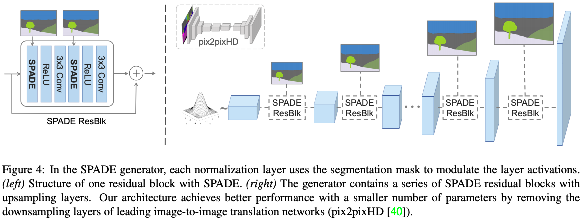
There are major differences in the architecture of GauGAN's generator and that of Pix2PixHD.

First, there is no downsampling involved. Downsampling layers build up semantic information. The authors instead opt for providing the semantic segmentation map directly as an input to each SPADE block (corresponding to different levels in the network).

Second, unlike Pix2PixHD, the upsampling is performed by a nearest neighbour resizing rather than by use of a transpose convolutional layer. Transpose convolutional layers have lost a lot of support due to their being susceptible to producing checkerboard artifacts in images. Practitioners have since started moving towards non-learnable upsampling followed by a convolutional layer instead. The authors have simply followed this trend.

The SPADE Normalization Layer

In the paper, the authors argue that unconditional normalization can lead to loss of semantic information. This form of normalization includes batch normalization and instance normalization.

Normalization in deep learning generally consists of three steps:

1. Computing the relevant statistics (like mean and standard deviation).
2. Normalizing the input by subtracting the mean and dividing this number by the standard deviation.
3. Re-scaling of the input $ y = \gamma x + \beta $ by use of learnable parameters $ \gamma, \beta $

Batch norm and instance norm differ in step 1, i.e how the statistics are computed. In batch norm, we compute the statistics across batches of images. In instance norm, we compute per image.

Here is an example to aid your imagination.

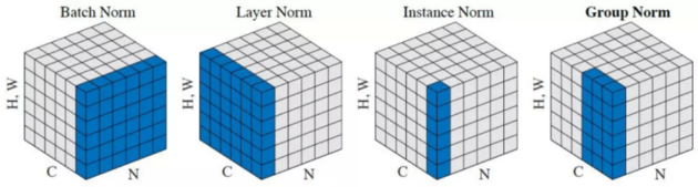
However, in SPADE, we modify batch norm (note that we still compute statistics across the mini-batch, per feature map) in such a way that we learn different sets of parameters for each pixel in the feature map, rather than learning a single set of parameters per channel. We do this directly by increasing the number of batch norm parameters to equal the number of pixels.

SPADE Generator Module

The authors introduce a SPADE Generator module, which is a small residual convolutional network which produces two feature maps: one corresponding to pixel-wise $ \beta's $ and another corresponding to pixel-wise $ \gamma's $ . Each pixel of these maps represents the parameters used to re-scale the value of the corresponding pixel in the feature map.

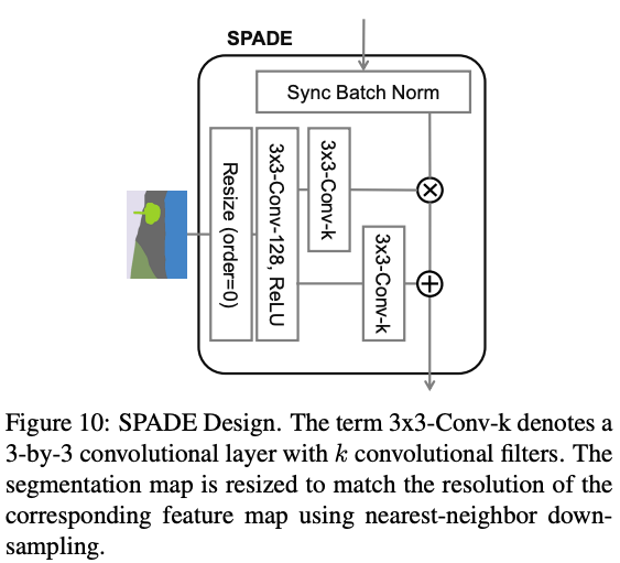
The above diagram might confuse some readers. We have a block called Batch Norm, which only performs computation of statistics. The computation of statistics in SPADE is similar to Batch Norm. The re-scaling is done later.

Synchronized normalization is called so in the context of how normalization is implemented on multi-GPU systems. Generally, if you have a batch size of say, 32 and you have 8 GPUs, PyTorch's nn.BatchNorm2d layer will compute statistics across 4 batches across each GPU separately and update the parameters. In synchronized Batch Norm, the statistics are computed over the entire 32 images. Synchronized normalization is useful when your per-GPU batch size is small, say 1 or 2. Computing statistics over small batches may produce very noisy estimates leading to jittery training.

The feature maps obtained as the out of the SPADE module are element-wise multiplied and added to the normalized input map.

Though not shown in the diagram in the paper, each convolutional layer is followed by Spectral Norm. For starters, Spectral Norm constrains the Lipschitz constant of the convolutional filters. A discussion of Spectral Norm is beyond the scope of this article. I have given a link to an article that talks about Spectral Norm.

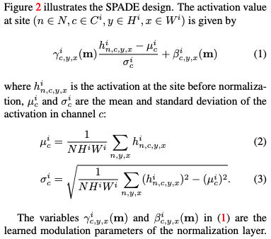
Here is the equations describing GauGAN.

Why does SPADE work?

The very first reason is that the input to GauGAN is a semantic map, which is further one-hot encoded.

This means that the GAN has to take regions of uniform values, precisely 1s, and produce pixels with diverse values so that they look like a real object. Having a different set of batch norm parameters for each pixel helps in tackling this task better than single set of batch norm parameters for the each channel in the feature map.

The authors also claim that SPADE leads to more discriminative semantic information. To support their claim, they take two image,s both of which have only a single label, sky for one and grass for the other. Though I find the following reasoning weak, I'll point it out for the sake of covering the paper judiciously.

Authors support their claim by giving an example where they take two images, containing only one label. Sky for one and Grass for the other. Applying convolutions to both these images produce different values but uniform ones. Authors then state that application of instance norm will turn both the different valued but uniform feature maps into a same-valued feature maps containing only zeros. This leads to loss of semantic information.

They then go on to show how the output of SPADE and Instance Norm differs given a semantic map containing the very same label.

However, this does not seem like an apple to apple comparison. First, the authors claim that the information gets decimated as a result of normalization. However, the normalization step in the SPADE and Instance Norm is identical. The place where they differ is the re-scaling step.

Second, in Pix2PixHD, the parameters of Instance Norm layer are non-learnable and Instance Norm is merely perform normalization ( $\gamma $set to 1 and  $\beta$ set to 0). However, in GauGAN, SPADE has learnable parameters.

Third, comparing Batch Norm and SPADE is a better comparison rather than that of Instance Norm and SPADE. This is because Instance Norm works with an effective batch size of 1, whereas both SPADE and Batch Norm can leverage larger batch sizes (Larger batch sizes lead to less noisier statistics estimates).

The Discriminator

Normally, the discriminator is a classifier network, with fully connected layers at the end and produces a single output between 0 and 1, given how realistic the image to the discriminator.

A multi-scale PatchGAN discriminator is a fully convolutional neural network. It outputs a feature map which is then averaged to get the "realistic-ness" score for the image. Being fully convolutional helps make the GAN process size invariant.

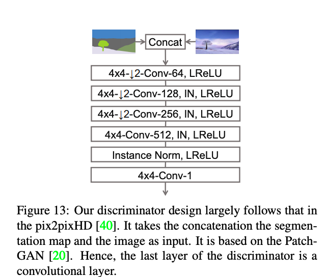
The paper claims that the Discriminator uses Spectral Norm just like the Generator. However, a look at the implementation shows that Instance Norm has been used. This is also reflected in the diagram.

The Encoder

Unlike vanilla GANs, GauGAN doesn't take a random noise vector, but only the semantic map. This means that given a single input semantic map, the output would always be deterministic. This goes against the spirit of Image Synthesis, as the ability to generate diverse outputs is highly valued. A GAN that merely reconstructs the input is only as good as an identity function. We do synthesis to generate data beyond our training data, and not just to recreate it using neural network.

For this purpose, the authors have devised an Encoder. The Encoder basically takes an image, encodes the image into two vectors. These two vectors are used as the mean and standard deviation of a normal Gaussian distribution. A random vector is then sampled from this distribution and then concatenated along with the input Semantic Map as an input to the generator.

As we sample different vectors, the synthesised results are also diversified as a result.

Style-Guided Image Synthesis

At the time of inference, this encoder can be used as a style guide for the image to be generated. We pass the  image to be used as the style guide through the encoder. The random vector generated is then concatenated with the input semantic map.

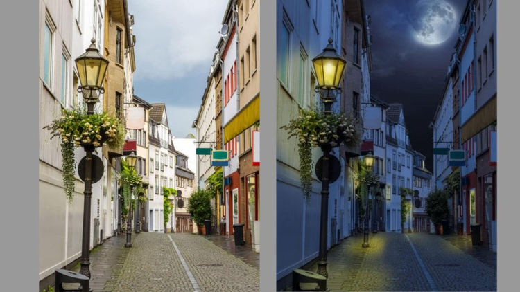
As we sample different values from the distribution (whose mean and standard deviation are predicted by the Encoder), we will be able to explore different modes of our data. For example, each random vector will produce an image with the same semantic layout but different modal features such as color, brightness etc.

Loss Function And Training

GauGAN's Loss Function consists of the following loss terms. I'm gonna go through each one of them as we go by.

Multiscale Adversarial Loss

GauGAN incorporates a hinge loss, that was also seen in papers like the SAGAN and Geometric GAN. The following is the loss function

Given an image generated by the generator, we create an image pyramid, resizing the generated image to multiple scales. Then, we compute the realness score using the discriminator for each of these scales and backpropagate the loss.

Feature Matching Loss

This loss encourages the GAN to produce the images which are not merely able to fool the generator, but the generated images should also have the same statistical properties as that of real images. In order to accomplish this, we penalize the L1 distance between the discriminator feature maps of the real images and the discriminator feature maps of the fake images.

Feature matching loss is computed for all the scales of the generated image.

$$ L_{FM} (G,D_k) =  \mathop{\mathbb{E}} {}_{s,x} \:\sum_{i=1}^{T}  \frac{1}{N_{i}}[||D^{(i)}_{k}{(s,x)} - D^{(i)}_{k}{(s,G(s))}||_1] $$

Here $k$ represents which image scale we are using. We use $T$ feature maps from the discriminator and $N_i$ is the normalizing constant for each feature map so that the L1 difference between every pair of feature maps has the same scale despite different number of filters in each feature map.

VGG Loss

This loss is similar to the above loss, the only difference being instead of using the discriminator to compute the feature maps, we use a VGG-19 pre-trained on Imagenet to compute the feature maps for real and the fake images. We then penalise the the L1 distance between these maps.

$$L_{VGG} (G,D_k) = \mathop{\mathbb{E}}_{s,x} \:\sum_{i=1}^{5}  \frac{1}{2^i}[||VGG{(x,M_{i})} - VGG(G(s), M_i)||_1] $$ $$where \: VGG(x,m) \:is\: the \:feature\: map \: m \:of \:  VGG19 \:when \:x \:is \:the \:input. \\\\ and \:M = \{``relu1\_1", ``relu2\_1"``relu3\_1"``relu4\_1"``relu5\_1"\} $$

Encoder Loss

Authors use a KL divergence Loss for the encoder
$$ L_{KLD} = D_{kl}(q(z|x) || p(z)) $$

In loss above, $q(z|x)$ is called the variational distribution, from which we draw out random vector $z$  given real image $x$ whereas $p(z)$ is the standard Gaussian distribution

Note that, while we can use a style image during inference, the ground truth of the segmentation map serves as our style image during training. This makes sense as the style of ground truth as well as the image we are trying to synthesize is the same.

You may recognise the above loss function as the the regularization loss term from Variational Auto-Encoder Loss.  With the Encoder, GauGAN behaves as a sort of Variational AutoEncoder, with the GauGAN playing the part of the decoder.

For this note familiar with Variational AutoEncoders, the KL divergence loss term acts as a regularizer for the Encoder.  This loss penalizes the KL divergence between the distribution predicted by our encoder and a zero mean Gaussian.

If not for this loss, the encoder could cheat by assigning a different random vector for each training example in our dataset, rather than actually learning a distribution that captures the modalities of our data. If this explanation is not clear to you, I recommend you to read more about Variational Autoencoders, the links for which I have provided below.

Conclusion

So, this wraps up our discussion of GauGAN's architecture and it's objective functions.

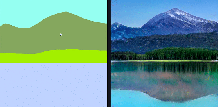
In the next part, we talk about how GauGAN is trained and how does it fare as compared to it's rival algorithms, especially it's predecessor Pix2PixHD. Till then, you can checkout the GauGAN web demo, which allows you to create random landscapes using a paint-like app.

Understanding GauGAN Series

• Part 1: Unraveling Nvidia's Landscape Painting GANs
• Part 2: Training on Custom Datasets
• Part 3: Model Evaluation Techniques
• Part 4: Debugging Training & Deciding If GauGAN Is Right For You

Further Reading

1. Batch Norm
2. VAE
3. GauGAN Demo
4. FID
5. Spectral Norm