Understanding GauGAN Part 4: Debugging Training & Deciding If GauGAN Is Right For You

Hey folks, welcome to Part 4 of our series on GauGAN. In the last three posts we covered the following topics:

1. The architecture and losses of GauGAN
2. How to set up a custom training (using the CamVid dataset as an example)
3. Understanding the different ways to evaluate GauGAN, problems that arise with evaluation metrics, and how GauGAN compares to other algorithms

In this part, we're going to talk about what you can do if your results are bad. We will also cover whether you can use GauGAN for something that you need in production.

In this post I will begin with what I call GAN First Aid Kit. This will cover basic tips and tricks of what to do in case your results are not good. However, if those issues still don't resolve, then maybe you need to step back and reconsider whether GauGAN is the right choice for you. Even if it's theoretically possible to get good results with GauGAN on the problem that you're trying to solve, it may require a huge dataset or a very high computational budget, which is going to increase the costs to a level that may not justify the investments.

Therefore in the second half of this article I will cover whether GauGAN makes sense from a business perspective or not. As exciting as GANs are, they are still in a very nascent stage of development. GauGAN, which claims to be the state of the art in semantic image generation, can still fall way short of the sort of behavior that is required from products that can be commercialized or shipped.

So, let's get started!

GAN First Aid Kit

So, you're training on your dataset and the results look absolutely terrible. What do you do? Are you under-fitting or over-fitting?

Loss Curves for GauGAN

Generally, GAN training curves are much harder to interpret than their discriminative cousins (like for object detection or image classification). This is because even for well-trained models, the loss rates converge to a range of somewhat constant values, and just keep oscillating between these values. For example, this is a loss plot for the discriminator and generator for a well-trained DCGAN model, which is a pretty effective GAN.

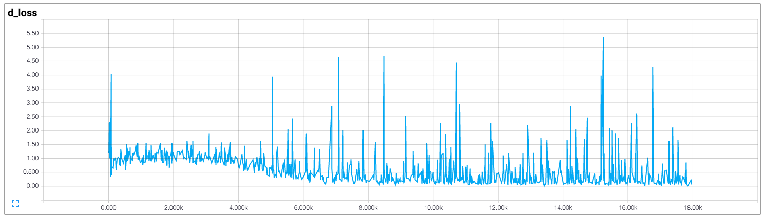
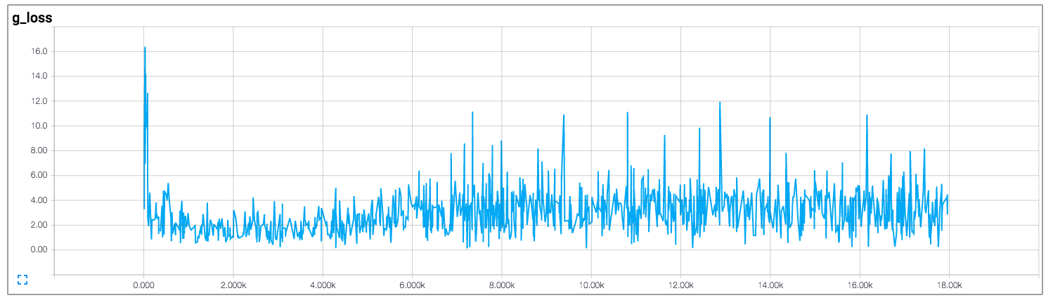
If you were to see such results while training an object detection model, you could definitely say that the training has saturated and the model has stopped learning. However, in the case of the GAN being trained above, learning was happening all the way through.

Why do GANs behave like this? It happens because unlike a normal deep learning algorithm where only one neural network is learning (and trying to decrease the loss), GANs instead have two neural networks competing against each other. For the mathematically inclined, two models are trained simultaneously to find a Nash equilibrium to a two-player non-cooperative game. However, each model updates its cost independently with no respect to another player in the game. Updating the gradient for both models concurrently cannot guarantee a convergence.

If the above line does not make any sense to you, understand this: if the loss of the discriminator decreases, then the loss of the generator must go up and vice-versa. The saturated loss for both of them means that both of them are effectively competing against each other. If that does not happen, our training cannot work.

If the discriminator totally decimates the generator, your generator can't learn anything. However, if the opposite happens, the generator can produce any gibberish and the discriminator will fail to recognize it as a fake. The discriminator is often represented as an adversary of the generator, but in reality, the generator only learns from the gradients backpropagated from the discriminator. In other words, the discriminator provides supervision to the generator, and tells it "Hey generator, this ain't real enough. Take these gradients and work better".

Imbalance between the generator and discriminator is therefore a problem that we need to address often with GANs.

Imbalance Between The Discriminator And The Generator

When we talk about imbalance between the discriminator and the generator, most likely we're going to deal with the discriminator overpowering the generator. If a discriminator fails then the generator is free to produce any random image without penalty, and thus the generator will fail as well.

So how do you establish that your discriminator has overpowered the generator? First, your discriminator loss would be driven to almost zero, whereas the generator loss will have a high value. Visually inspecting your training results might also show that your generator is mostly producing noise rather than realistic images. One should also check the classification accuracy of the discriminator; such an imbalance is likely if the discriminator accuracy is more than 80-85% for a sizeable period of time.

How To Restore Balance

There are a few things you can try to overcome this problem. Consider doing the following, in order:

• The first and very intuitive step is to make the generator more powerful by increasing the value of number of filters in the generator (--ngf) and the number of layers (--n_downsample_layers).
• Decrease the learning rate for the generator. This may help it learn better as it can explore the loss surface more thoroughly rather than shooting around. You can also combine a slower learning rate with more update steps for the generator than the discriminator. For example, consider updating the generator twice for every update of the discriminator.
• Use soft labels for real images. Although in the beginning of training the real images have their labels set to 1 when computing the discriminator loss, instead try denoting them with 0.9 (or maybe a random number between 0.7 and 1.2). Why exactly does this work? It was observed that with hard labels (1), the discriminator can become over-confident and end up relying only on a subset of features to classify an example. This may cause the generator to focus only on those features to fool the discriminator, causing the training to crash.
• Use spectral normalization in your discriminator. GauGAN's code repo uses spectral norm for both the generator and discriminator by default.
• Add noise to both your real data and generated data before sending it to the discriminator. How does it help? It helps because it's often observed that data distributions, despite being high-dimensional, live on low-dimensional manifolds which makes it much easy for the discriminator to find a hyperplane that perfectly separates the real data from the fake data. If this line doesn't make sense to you, don't worry. It just means that noise prevents the discriminator from completely steamrolling the generator.
• Lastly, if you observe that your generator has stopped improving, try making the discriminator more powerful using the --ndf flag. Sometimes the generator stops learning because the supervision isn't good enough.

Other Losses in GauGAN

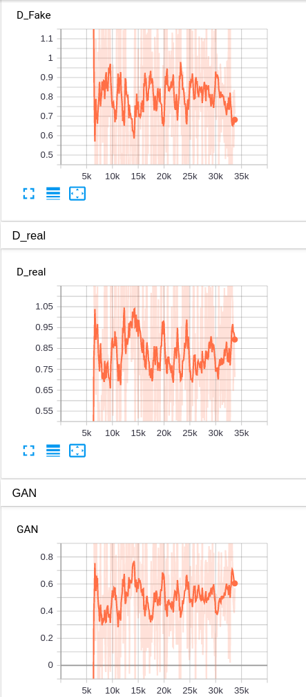
Apart from the main adversarial losses, GauGAN also uses Feature Matching Loss and Perceptual Loss. (I did not train with KL divergence loss).

This is what each of these losses look like for stable training.

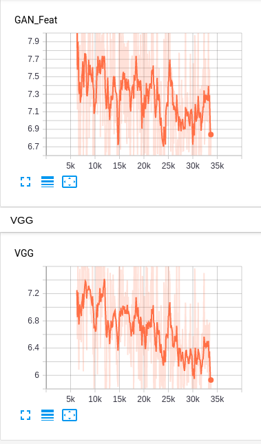
I want you to be a bit wary of the decreasing Perceptual Loss (VGG Loss). The VGG loss is decreasing on the training set, but you may also want to see it on the test set/validation set. Since the adversarial losses stabilize during training, gradient descent tends to reduce the net loss by reducing the perceptual loss. You have to be careful in case this leads to overfitting, and accordingly reduce its contribution to the loss term by rescaling it.

Unfortunately, the code for GauGAN does not provide options to set scales for the weights and one has to do this by modifying the code. This can be done by playing around with the code defined in the functions run_generator_one_step and run_discriminator_one_step in the file pix2pix_trainer.py.

  def run_generator_one_step(self, data):
        self.optimizer_G.zero_grad()
        g_losses, generated = self.pix2pix_model(data, mode='generator')
        g_loss = sum(g_losses.values()).mean()
        g_loss.backward()
        self.optimizer_G.step()
        self.g_losses = g_losses
        self.generated = generated

The object g_loss returned in line 4 is a dictionary consisting of keys GAN (GAN loss), GAN_Feat (Feature Matching Loss), and VGG (VGG loss). Multiply these values by numbers to scale them. For example, let's say I want to scale VGG loss by 2. So, my function would look like:

def run_generator_one_step(self, data):
        self.optimizer_G.zero_grad()
        g_losses, generated = self.pix2pix_model(data, mode='generator')
        # scale modification
        g_losses['VGG'] *= 2
        g_loss = sum(g_losses.values()).mean()
        g_loss.backward()
        self.optimizer_G.step()
        self.g_losses = g_losses
        self.generated = generated

    def run_discriminator_one_step(self, data):
        self.optimizer_D.zero_grad()
        d_losses = self.pix2pix_model(data, mode='discriminator')
        d_loss = sum(d_losses.values()).mean()
        d_loss.backward()
        self.optimizer_D.step()
        self.d_losses = d_losses

Similarly, the object d_losses returned in line 3 contain the keys D_real and D_fake for discriminator losses on real and fake images respectively.

Batch Size

The larger the batch size, the better your results should be since small batches often provide a very noisy estimate of the statistics of the data distribution. The authors use a batch size of 128, which requires an Octa-GPU machine with each GPU having 16 GB VRAM. Therefore, training GauGAN can be pretty expensive.

If you are using GauGAN for your business, or if you are short on resources, maybe it's not the best time to use GauGAN. In the next section, I will cover how to determine whether you should reconsider your decision to use GauGAN – especially from a business perspective.

Is GauGAN Right for You?

Here's the meat of this post. Is GauGAN right for you? While working at MathWorks I learned many things about the business side of implementing DL algorithms. As far as these are concerned, GauGAN is pretty demanding for the following reasons.

Your problem needs to be the right kind of difficult

What do I mean by this? Well, the very first thing you have to consider is that GauGAN has its limits. The technology is still very much in its nascent stage. GauGAN is adept at synthesizing textural details of various things. Boundaries are generally handled well as long as they're not between objects of the same class. While instance segmentation maps help in this case, two overlapping objects of similar classes can often morph into one distorted object.

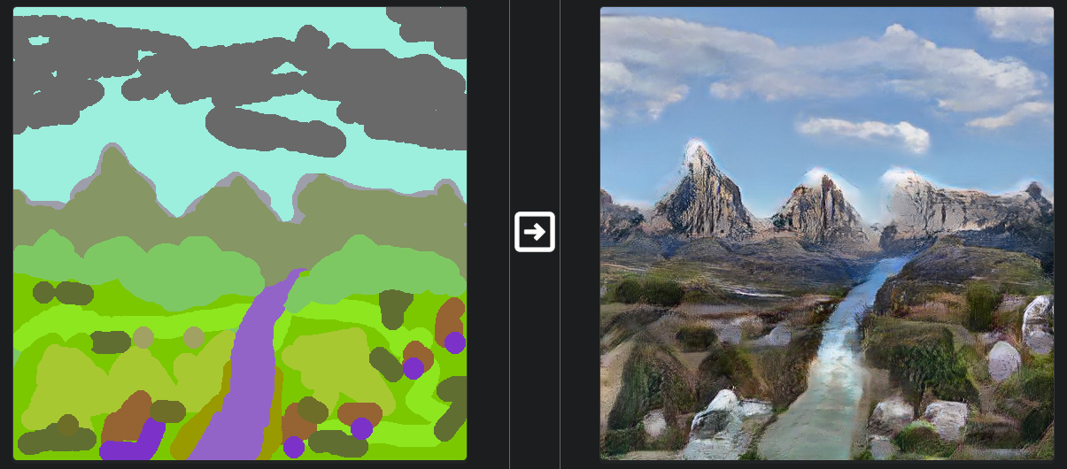
Nvidia used the Flickr landscapes dataset for their GauGAN demos. Landscapes mostly consist of texture, e.g. the texture of a mountain, the sky, the sea, etc.

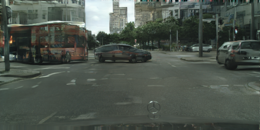
However, GauGAN may struggle with dense traffic scenes which require it to create objects with a lot of spatial detail crammed into a small area. Take the cars in the following image, for example.

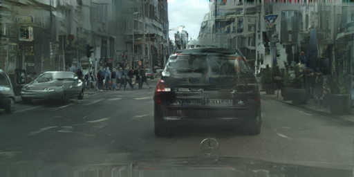
Unlike filling in texture, which can have a considerable degree of randomness, structural components of objects need to be rendered in a more constrained manner. While GauGAN can perform well if these spatial details are sparse and spread over a large area of the image (like having only a human body figure to render in front of the camera), it may produce blurry objects when these objects should have lot of detail confined to a small portion of the image (like a crowd of pedestrians in all sorts of poses).

So, if your problem has sparse structural details (like single human figures or close-up car pictures) or textural details (like landscapes or microscopic bacteria stains) ,use GauGAN. Otherwise, you may want to wait for the technology to improve.

You need compute resources

GauGAN requires a lot of resources. I mean a lot. Batch size can make or break your training, and larger batch sizes require you to have GPUs with large memory. Of course, this will also depend on your image size and the complexity of your problem.

If you are working with images of bacteria stains of sizes 128 x 128, you can easily fit a large enough batch in a 24 GB GPU system. However, if you are dealing with imagery to the scale of 1024 x 768, get ready to shell out for a lot of resources. With its default parameters, you will need about 16 GB of memory to fit just a single example.

You could try increasing the size of an image using bilinear upsampling post-generation. Or if you feel your task is not too hard, try reducing the number of filters in the generator and the discriminator and see whether you can get by with marginal losses in performance.

Also owing to small batch sizes, getting the right model may take longer due to longer training times. GANs can be notoriously hard to get working, and may need a lot of experimentation to work correctly. Count yourself lucky if your task matches one of the tasks for which pre-trained models have been provided, since the same set of hyperparameters might work.

So time is another resource you need to watch out for, especially if your problem is different from the tasks that pre-trained models have provided for.

You need the right kind of data

If you have followed this series, you will realize that I have used the CamVid dataset for demonstration purposes. I chose it for a couple of reasons. It's a small enough dataset, only 700 images to train so you can get results quickly. Second, and as you may have already noticed, the results can be pretty bad. The CamVid dataset has almost all things going wrong for it, almost reminding me of Murphy's Law.

Here is one of the best results from CamVid.

Here is one of the worst. Yep, it's bad.

So, when you are looking at acquiring data for your problem, make sure it's not like CamVid because of the following reasons.

It's too small a dataset. GauGAN, like any deep learning network, needs a large amount of data. For complex scenarios like traffic scenes, a good figure for the training set would be around 5000-10000 examples. By comparison, CamVid I trained had 630. Meh. I've worked with Cityscapes (3000 images) as well as the Intel Indian Driving Dataset (7000 images). The training performance increases with the amount of data.  

The amount of data required to reach a good solution would also change with the complexity of the task at hand. For bacteria stains, you could do with only 2000 examples. Even datasets like Cityscapes are much simpler than the Indian driving dataset, which contains more types of vehicles, locations (such as alleys with unpaved roads), and more types of surfaces (like muddy surfaces besides roads).

Pre-trained models are your best bet to judge how much data you need. Gauge the complexity of your task by looking at the datasets on which pre-trained models have been provided and extrapolate the amount of data needed for your task accordingly.

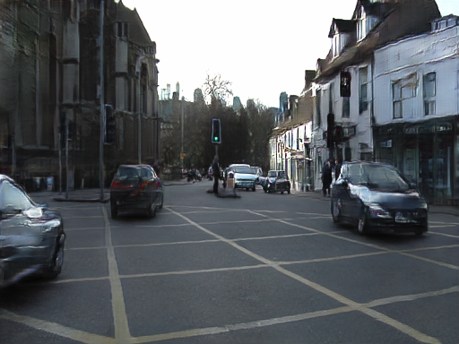
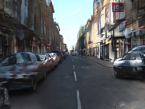
It's not diverse enough. The problem with CamVid is that instead of having diverse images like Cityscapes, it's a dataset which contains subsequent frames from only four drives through Cambridge. This means that there is very little difference between subsequent frames, or they are highly correlated. For example, consider these three consecutive frames:

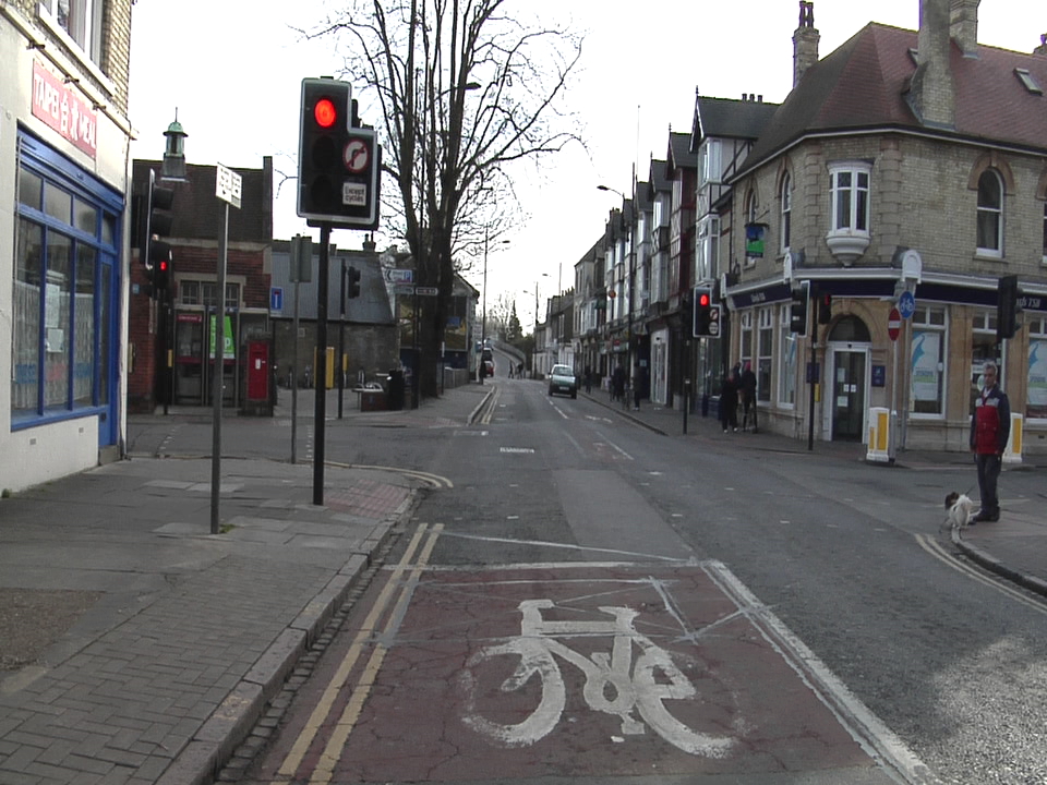
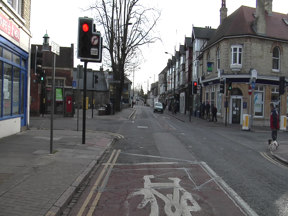
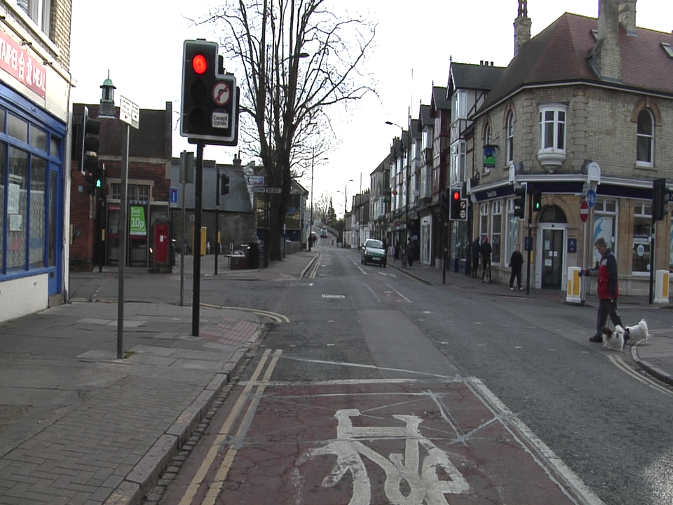
At worst, the vehicle is stationary and you have almost the same frames exactly.

This gives us a deceptive idea that we have around 640 images, whereas the truth it that many of these frames have repetitive information in them which is stifling GauGAN.

Some modes are much more frequent than others. When I say your data should be diverse, I mean it should cover all possible ways your objects may appear. Imbalances may cause GauGAN to perform poorly on rarer orientations. For example, in datasets cars are mostly seen from the back and front, while views of cars from the side are very rare. This results in the algorithm trying to paint the cars in a side orientation as one in front/back orientation. For example:

The training and test sets are too similar. Random sampling frames from consecutive video scenes can leave your test set incredibly similar to the training set, and give you a deceptively good performance. For example, consider randomly sampling from the CamVid data to create your test set.

Consider the three frames you saw above. Let's say the second frame gets sampled into our test set. The algorithm will perform well on it since the second frame is so similar to the first and third frames. Our learning algorithm is overfit, even though it's not evident in the training results.

In CamVid a better metric would be to train on three driving scenarios and test it on the fourth. Unfortunately this also does not work quite well since our dataset size is too low.

Conclusion

And that's a wrap for our GauGAN series. The idea of the series was to get you up to speed on a recent state of the art GAN, tell you its problems and how you could try to solve them. Stuck with another problem related to GauGAN? Generated some cool results using it? Or did you solve an open problem we mentioned above? Feel free to hit the comment section. Until then, here are a few resources for you to further your understanding of GANS.

1. Improved Techniques for Training GANs
2. How to Train a GAN? Tips and tricks to make GANs work
3. 10 Lessons I Learned Training GANs for one Year

Understanding GauGAN Series

• Part 1: Unraveling Nvidia's Landscape Painting GANs
• Part 2: Training on Custom Datasets
• Part 3: Model Evaluation Techniques
• Part 4: Debugging Training & Deciding If GauGAN Is Right For You