Earlier this year, we showcased the PixRay project's PixelDrawer to demonstrate how, with nothing but a text prompt, we can generate a unique and creative piece that is accurate to the provided description. PixRay can also be used to create colorful and detailed, albeit slightly cartoonish and surreal, art. The problem with this being the uncanny valley: the images generated with these models are accurate to the text prompt in terms of meaning, but they often do not resemble reality.

Thus, the goal of generating pieces so photorealistic that they can fool both AI and human actors is an interesting challenge, and doing so accurately and generally to meet the potential scope of a random text prompt is even more difficult. Interpreting the meaning of a string and translating that message to an image is a task that even humans can struggle with. This is largely why text to visual models like CLIP tend to pop up so frequently in research on this subject.

In this article, we will examine OpenAI's GLIDE, one of the many exciting projects working towards generating and editing photorealistic images using text-guided diffusion models. We will first break down how GLIDE's diffusion model based framework runs under the hood, then walk through a code demo for running GLIDE on a Gradient Notebook.

GLIDE

Architecture

The GLIDE architecture can be boiled down to three parts: an Ablated Diffusion Model (ADM) trained to generate a 64 x 64 image, a text model (transformer) that influences that image generation through a text prompt, and an upsampling model that takes our small 64 x 64 images to a more interpretable 256 x 256 pixels. The first two components interact with one another to guide the image generation process to accurately reflect the text prompt, and the latter is necessary to make the images we produce more easy to interpret.

The roots of the GLIDE project lie in another paper released in 2021, which showed that ADM approaches could outperform contemporarily popular, state-of-the-art generative models in terms of image sample quality. The GLIDE authors used the same ImageNet 64 × 64 model as Dhariwal and Nichol for the ADM, but opted to increase the model width to 512 channels. This results in around 2.3 billion parameters for the ImageNet model. Unlike Dhariwal and Nichol, however, the GLIDE team wanted to be able to influence the image generation process more directly, so they paired the visual model with an attention-enabled transformer.

By processing the text input prompts, GLIDE enables some measure of control over the output of the image generation process. This is done by training the transformer model on a sufficiently large dataset (the same used in the DALL-E project) consisting of images and their corresponding captions. To condition on the text, the text is first encoded into a sequence of K tokens. These tokens are then fed into a transformer model. The transformer's output then has two uses. First, the final token embedding is used in place of the class embedding for the ADM model. Second, the last layer of the token embeddings - a sequence of feature vectors - is projected separately to the dimensions for every attention layer in the ADM model and concatenated to the attention context of each. In practice, this allows for the ADM model to use its learned understanding of the inputted words and their associated images to generate an image from novel combinations of similar text tokens in a unique and photorealistic manner. This text-encoding transformer uses 24 residual blocks of width 2048, and has roughly 1.2 billion parameters.  

Finally, the upsampler diffusion model also has roughly 1.5 billion parameters, and differs from the base model in that its text encoder is smaller, having a width of 1024 and 384 base channels. As the name implies, this model helps upscale the sample to raise the interpretability for machine and human actors.

The Diffusion Model

GLIDE leverages its own implementation of the ADM (ADM-G for "guided") to perform its image generation. The ADM-G can be thought of as an adaptation of the diffusion U-net model.

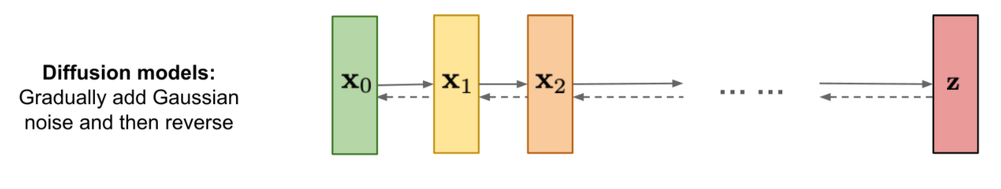
A diffusion U-net model differs significantly from the more popular VAE, GAN, and transformer based image synthesis techniques. They create a Markov chain of diffusion steps to incrementally introduce random noise to the data and then they learn to reverse the diffusion process, and reconstruct the desired data samples from the noise alone.

It works in two stages: forward diffusion and backward diffusion. Given a data point from the real distribution of the sample, the forward diffusion process adds a small amount of noise to the sample for a predefined set of steps. As the steps get larger and approach infinity, the sample will lose all of its distinguishable features and the sequence will begin to mimic an isotropic gaussian curve. During the backward diffusion process, the diffusion model sequentially learns to reverse the effect of the added noise to the images, and guide the generated image towards its original form by trying to approximate the original input sample distribution. A perfected model would be able to do so from a true gaussian noise input and a prompt.  

The ADM-G differs from the process above in that a model, either CLIP or a specialized transformer, influences the backward diffusion step using the inputted text prompt tokens.

CLIP vs. Classifier-free Guidance

As part of the development of the GLIDE image synthesizer, the researchers sought to create a novel, improved methodology for influencing the generation process. Typically, the "classifier is first trained on noised images, and during the diffusion sampling process, gradients from the classifier are used to guide the sample towards the label" (Source). This is where a model like CLIP typically would be used instead. CLIP learns visual concepts from natural language supervision, and can impart those learned concepts to the image synthesis process. The trade off, however, is that using CLIP is computationally expensive. At the same time, a precedent for not using a classifier for guidance was shown by Ho & Saliman (2021). They demonstrated that comparable image quality could be achieved by "interpolating between predictions from a diffusion model with and without labels" (Source). This was dubbed classifier-free guidance.

# Create a classifier-free guidance sampling function
def model_fn(x_t, ts, **kwargs):
    half = x_t[: len(x_t) // 2]
    combined = th.cat([half, half], dim=0)
    model_out = model(combined, ts, **kwargs)
    eps, rest = model_out[:, :3], model_out[:, 3:]
    cond_eps, uncond_eps = th.split(eps, len(eps) // 2, dim=0)
    half_eps = uncond_eps + guidance_scale * (cond_eps - uncond_eps)
    eps = th.cat([half_eps, half_eps], dim=0)
    return th.cat([eps, rest], dim=1)

Following in these findings, GLIDE's classifier free guidance serves as a gradient function that behaves similarly to the model (see code above). This is a parameter for the p_sample_loop (training) function that can be used to force the diffusion model to use its own learned understanding of the inputs to influence the image generation procedure.

Overall for this task, the authors of GLIDE found classifier-free guidance to be more effective than using CLIP. The reasons for this are two fold. First, a single model can use its own knowledge to guide the synthesis, rather than having to do so via interpretations of a separate classification model. Second, it simplifies guidance when conditioning on information that is difficult to predict with a classifier (such as text). As a result, when put up to a human test of quality, images generated with the classifier-free guidance were generally described as being higher quality and more accurate to the caption when compared to images generated without guidance or with CLIP.

The authors also surmise that the publicly available CLIP models are not trained on sufficiently noised data, and that the noised intermediate images encountered during sampling are out-of-distribution for them. This could potentially lead to some of the differences in perceived capabilities between the two methods.

You can use the clip_guided.ipynb and text2im.ipynb notebooks to test their abilities yourself!

Capabilities

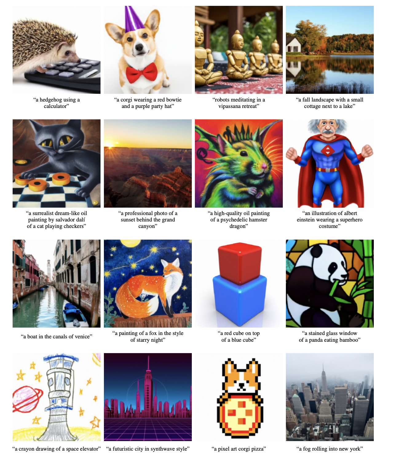
Image Generation

The most popular and common use case for GLIDE will undoubtedly be its potential for image synthesis. While the images are small and GLIDE struggles with animal/human shapes, the potential for one shot image generation is near limitless. Not only can it generate images of animals, celebrities, landscapes, buildings and much more, but it can also do so in different art styles or photorealistically. As you can see from the samples above, the authors of the paper argue GLIDE is capable of understanding and adapting a wide variety of textual inputs into image format.

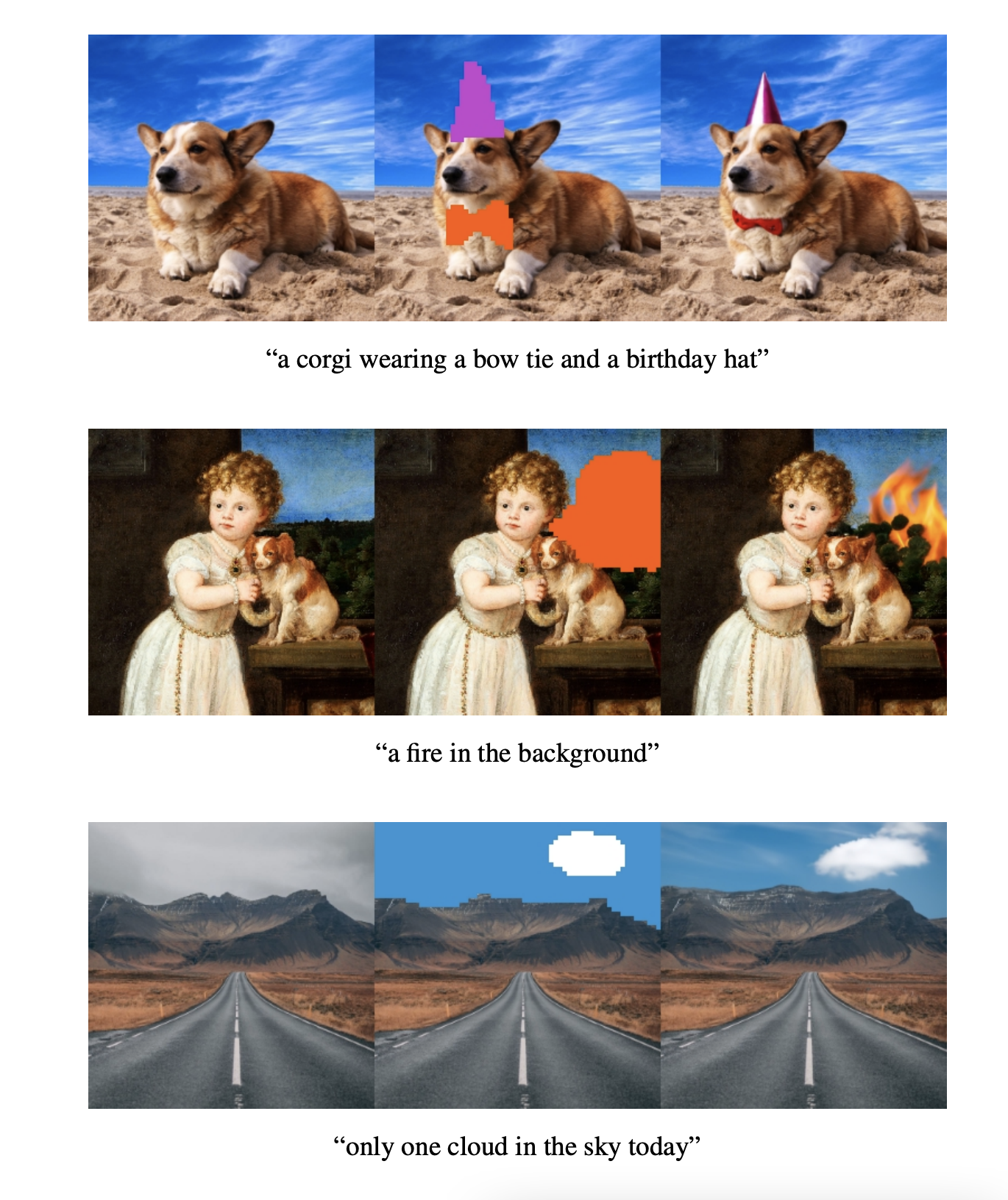
Inpainting

Arguably, the more interesting application of GLIDE is its automated photo inpainting. GLIDE is capable of taking in an existing image as input, process it with the text prompt in mind for areas that need to be edited, and can actively make additions to an image to those regions with ease. To achieve even better results, GLIDE needs to be used in conjunction with an editing model, like SDEdit. In the future, applications leveraging abilities such as this are potentially key for creating code-less methods for image editing.

Code Demo

We have created a fork of the GLIDE repo containing demo notebooks that have been optimized to run on Gradient for your convenience, so be sure to check them out! You can also access and fork the demo Notebook directly from Gradient. There are three notebooks in the notebooks directory of the repo, each focused on a different task. For classifier free guidance on image generation: use the text2im.ipynb, for CLIP guidance: use clip_guided.ipynb, and for inpainting an existing photo: use inpaint.ipynb.

Once you have everything set up, let's get started by going into the inpaint.ipynb file. This is the notebook you can use to input your own images to be edited by the inpainting model. We are going to walkthrough the inpainting notebook for this demo because it is arguably the most novel use of the ADM-G shown in the paper. The other notebooks will not be covered in this blogpost, but should be simple to understand due to their high degree of similarity to the one covered in this blog.

Let's jump into it.

!pip install git+https://github.com/gradient-ai/glide-text2im

Be sure to run the first cell. This will install the Github repo as a Python package for us to use in the demo. If you are on Gradient, make sure you are using the gradient-ai Github fork in the install if you want the code to run.

from PIL import Image
from IPython.display import display
import torch as th

from glide_text2im.download import load_checkpoint
from glide_text2im.model_creation import (
    create_model_and_diffusion,
    model_and_diffusion_defaults,
    model_and_diffusion_defaults_upsampler
)

Here we have our imports. The glide_text2im library you just installed has provided a lot of helpful functions for us to create our model and get started.

# This notebook supports both CPU and GPU.
# On CPU, generating one sample may take on the order of 20 minutes.
# On a GPU, it should be under a minute.

has_cuda = th.cuda.is_available()
device = th.device('cpu' if not has_cuda else 'cuda')

Run this cell to make sure that your GPU is being used by PyTorch during the training process.

# Create base model.
options = model_and_diffusion_defaults()
options['inpaint'] = True
options['use_fp16'] = has_cuda
options['timestep_respacing'] = '100' # use 100 diffusion steps for fast sampling
model, diffusion = create_model_and_diffusion(**options)
model.eval()
if has_cuda:
    model.convert_to_fp16()
model.to(device)
model.load_state_dict(load_checkpoint('base-inpaint', device))
print('total base parameters', sum(x.numel() for x in model.parameters()))

Here we are loading in the inpaint base model, which will perform the inpainting. First, we use the provided function model_and_diffusion_defaults() to create our configuration settings for the base model. Next, create_model_and_diffusion() uses those params to create the ImageNet and diffusion models to be used. model.eval() then puts the model in evaluation mode so we can use it for inference, while model.to(device) ensures that operations by the model will be performed with the GPU. Finally, model.load_state_dict() loads the checkpoint provided by OpenAI for the baseline inpaint model.

# Create upsampler model.
options_up = model_and_diffusion_defaults_upsampler()
options_up['inpaint'] = True
options_up['use_fp16'] = has_cuda
options_up['timestep_respacing'] = 'fast27' # use 27 diffusion steps for very fast sampling
model_up, diffusion_up = create_model_and_diffusion(**options_up)
model_up.eval()
if has_cuda:
    model_up.convert_to_fp16()
model_up.to(device)
model_up.load_state_dict(load_checkpoint('upsample-inpaint', device))
print('total upsampler parameters', sum(x.numel() for x in model_up.parameters()))

Similar to above, we now need to load in the upsample model. This model will take the sample generated by the base model, and upsample it to 256 x 256. We use 'fast27' for the timestep_respacing here to quickly generate our enlarged photo from the sample. Just like with the baseline, we use the parameters to create our upsample model and upsample diffusion model, set the upsample model to evaluation mode, and then load in the checkpoint for the inpainting upsample model to our model_up variable.

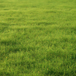
Here is the sample 'grass.png' we will be using in the demo. This image will be painted over with whatever you input as the prompt. Our sample input is going to be "a small house on fire," but feel free to change it how you please.  You can also upload your own images and test them by changing the path in the source_image_256 and source_image_64 variable assignment functions shown below.

# Sampling parameters
prompt = "a small house on fire"
batch_size = 1
guidance_scale = 5.0

# Tune this parameter to control the sharpness of 256x256 images.
# A value of 1.0 is sharper, but sometimes results in grainy artifacts.
upsample_temp = 0.997

# Source image we are inpainting
source_image_256 = read_image('grass.png', size=256)
source_image_64 = read_image('grass.png', size=64)

# The mask should always be a boolean 64x64 mask, and then we
# can upsample it for the second stage.
source_mask_64 = th.ones_like(source_image_64)[:, :1]
source_mask_64[:, :, 20:] = 0
source_mask_256 = F.interpolate(source_mask_64, (256, 256), mode='nearest')

# Visualize the image we are inpainting
# show_images(source_image_256 * source_mask_256)

This cell contains the final steps for setting up the image generation with GLIDE. Here, we establish our prompt, batch_size, and guidance_scale parameters. Notably, the prompt determines what the inpainter will try to add or remove from the image, and the guidance_scale affects how strongly the classifier free guidance will try to act on the image.  Finally, we generate our source masks. These are used to identify the regions in the photo to be inpainted.

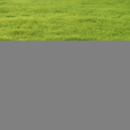
In the inpaint.ipynb, we also need to load in our sample image as both a 64 x 64 and 256 x 256 image. We can then use the 64 x 64 version to create our mask to identify the areas for inpainting in our sample in both sized images.

##############################
# Sample from the base model #
##############################

# Create the text tokens to feed to the model.
tokens = model.tokenizer.encode(prompt)
tokens, mask = model.tokenizer.padded_tokens_and_mask(
    tokens, options['text_ctx']
)

# Create the classifier-free guidance tokens (empty)
full_batch_size = batch_size * 2
uncond_tokens, uncond_mask = model.tokenizer.padded_tokens_and_mask(
    [], options['text_ctx']
)

# Pack the tokens together into model kwargs.
model_kwargs = dict(
    tokens=th.tensor(
        [tokens] * batch_size + [uncond_tokens] * batch_size, device=device
    ),
    mask=th.tensor(
        [mask] * batch_size + [uncond_mask] * batch_size,
        dtype=th.bool,
        device=device,
    ),

    # Masked inpainting image
    inpaint_image=(source_image_64 * source_mask_64).repeat(full_batch_size, 1, 1, 1).to(device),
    inpaint_mask=source_mask_64.repeat(full_batch_size, 1, 1, 1).to(device),
)

# Create an classifier-free guidance sampling function
def model_fn(x_t, ts, **kwargs):
    half = x_t[: len(x_t) // 2]
    combined = th.cat([half, half], dim=0)
    model_out = model(combined, ts, **kwargs)
    eps, rest = model_out[:, :3], model_out[:, 3:]
    cond_eps, uncond_eps = th.split(eps, len(eps) // 2, dim=0)
    half_eps = uncond_eps + guidance_scale * (cond_eps - uncond_eps)
    eps = th.cat([half_eps, half_eps], dim=0)
    return th.cat([eps, rest], dim=1)

def denoised_fn(x_start):
    # Force the model to have the exact right x_start predictions
    # for the part of the image which is known.
    return (
        x_start * (1 - model_kwargs['inpaint_mask'])
        + model_kwargs['inpaint_image'] * model_kwargs['inpaint_mask']
    )

# Sample from the base model.
model.del_cache()
samples = diffusion.p_sample_loop(
    model_fn,
    (full_batch_size, 3, options["image_size"], options["image_size"]),
    device=device,
    clip_denoised=True,
    progress=False,
    model_kwargs=model_kwargs,
    cond_fn=None,
    denoised_fn=denoised_fn,
)[:batch_size]
model.del_cache()

# Show the output
show_images(samples)

Now that set up is complete, this cell contains everything needed to create the 64 x 64 inpainted image. First, we create the text tokens to feed into the model from the prompt, and use the batch_size to generate the conditional text tokens and mask for our model. Next, we create an empty sequence of tokens to serve as the classifier-free guidance text tokens and a corresponding mask. We then concatenate the two sets of tokens and masks in the model_kwargs dictionary, along with our inpaint image and its corresponding image mask. model_kwargs is then used, along with the input tensor for the image and our inputted number of steps, to create the model_fn. model_fn is used to perform inpainting by sampling from the diffusion model to generate the image, but replacing the known region of the image with a sample from a noised version of the context after each sampling step.  This is done by finetuning the model to erase random regions of the training examples, and inputting the remaining portions into the model with a mask channel as additional conditioning information (Source). In practice, the generator learns to add the information suggested by the text prompt tokens to the masked portion of image.

Once this cell completes running, it will output a 64 x 64 generated image that contains the inpainting changes specified in your prompt. This image is then used by the upsample model to create our final 256 x 256 image.

##############################
# Upsample the 64x64 samples #
##############################

tokens = model_up.tokenizer.encode(prompt)
tokens, mask = model_up.tokenizer.padded_tokens_and_mask(
    tokens, options_up['text_ctx']
)

# Create the model conditioning dict.
model_kwargs = dict(
    # Low-res image to upsample.
    low_res=((samples+1)*127.5).round()/127.5 - 1,

    # Text tokens
    tokens=th.tensor(
        [tokens] * batch_size, device=device
    ),
    mask=th.tensor(
        [mask] * batch_size,
        dtype=th.bool,
        device=device,
    ),

    # Masked inpainting image.
    inpaint_image=(source_image_256 * source_mask_256).repeat(batch_size, 1, 1, 1).to(device),
    inpaint_mask=source_mask_256.repeat(batch_size, 1, 1, 1).to(device),
)

def denoised_fn(x_start):
    # Force the model to have the exact right x_start predictions
    # for the part of the image which is known.
    return (
        x_start * (1 - model_kwargs['inpaint_mask'])
        + model_kwargs['inpaint_image'] * model_kwargs['inpaint_mask']
    )

# Sample from the base model.
model_up.del_cache()
up_shape = (batch_size, 3, options_up["image_size"], options_up["image_size"])
up_samples = diffusion_up.p_sample_loop(
    model_up,
    up_shape,
    noise=th.randn(up_shape, device=device) * upsample_temp,
    device=device,
    clip_denoised=True,
    progress=False,
    model_kwargs=model_kwargs,
    cond_fn=None,
    denoised_fn=denoised_fn,
)[:batch_size]
model_up.del_cache()

# Show the output
show_images(up_samples)

Finally, now that we have generated our initial image, it's time to use our diffusion upsampler to get the image in 256 x 256. First, we reassign our tokens and mask using model_up.  We then pack the samples variable representing our generated image; the tokens and mask, the inpainting image, and inpainting mask together as our model_kwargs. We then use our diffusion_up model to upsample the image (now stored as low_res in the kwargs) for the "fast" 27 steps.

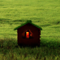
After running all of these steps on a Gradient Notebook, we were able to generate this 256 x 256 inpainting. As you can see, it has managed to capture the spirit of the prompt ("a small house on fire"), by adding the cottage looking portion with a flame shining through the window.  It also seems to have identified that the original sample was at an angle aimed towards the ground. The COCO dataset the models were trained on likely didn't have any images of houses at such an angle. To remedy this, a patch of more horizontal grass was added for the cottage to stand on.

As you can see, GLIDE is not without its problems. Though it can create photorealistic images, the scope of what sorts of images can be made is limited. In our testing, we found GLIDE struggling when working with images of real people. Faces in particular were difficult for GLIDE to work with, and it often would morph and twist a face on inpainting tasks rather than making the suggested changes. Other problems include the presence of artifacts that occasionally pop up in otherwise realistic images. Finally, the cost of running the model is relatively high just for 256 x 256 images. It's reasonable to assume that this would only exponentially increase if we were to upsample further or use the expensive CLIP to guide the process.

Closing thoughts

Now that we have walked through the process, you should now understand the basics of how GLIDE works, understand the scope of its capabilities in image generation and in-image editing, and can now implement it on a Gradient notebook. We encourage you to try this tutorial out, and see what interesting images you can get out of the neat model.

This is a part of a unofficial series on text guided image generation. Be sure to check out the walkthrough for implementing PixRay's CLIPit-PixelDraw next if art and image generation is a subject of interest.