Neural Machine Translation is the practice of using Deep Learning to generate an accurate translation of text from one language to another. This means training a deep neural network to predict the likelihood of a sequence of words as a correct translation.

The uses for such a technique are near infinite. Today, we have translators capable of nearly instantaneous and relatively accurate translation of entire webpages written in other languages. We can point a camera at a piece of text and use augmented reality to replace the text with a translation. We can even dynamically translate live speech to text in other languages. This capability has largely enabled technological globalization, and wouldn't be possible without the concept of sequence to sequence neural machine translation.

The first Seq2Seq (sequence to sequence) translator was introduced by researchers at Google in 2014. Their invention has radically changed the translation scene, with popular services like Google Translate growing to enormous levels of accuracy and accessibility to meet the internet's needs.  

In this blog post, we will break down the theory and design of Seq2Seq translation. Then, we will walk through an augmented version of the official PyTorch guide to Seq2Seq translation from scratch, where we will first improve the original framework before demonstrating how to adapt it to a novel dataset.

Seq2Seq Translators: How do they work?

A Seq2Seq translator operates in a, for deep learning, relatively straightforward manor. The goal of this class of models is to map a string input of a fixed-length to a paired string output of fixed length, in which these two lengths can differ. If a string in the input language has 8 words, and the same sentence in the target language has 4 words, then a high quality translator should infer that and shorten the sentence length of the output.

Design Theory:

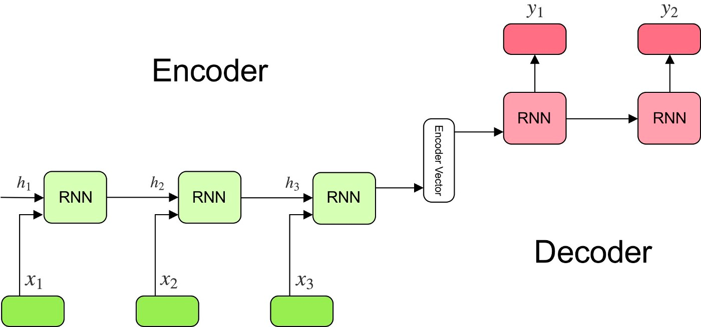
Seq2Seq translators typically share a common framework. The three primary components of any Seq2Seq translator are the encoder and decoder networks and an intermediary vector encoding between them. These networks are often Recurrent Neural Networks (RNN), but frequently they are made up with the more specialized Gated Recurrent Unit (GRU) and Long Short Term Memory (LSTM). This is to limit a potential vanishing gradient from affecting the translation.

The encoder network is a series of these RNN units. It uses these to sequentially encode the elements from the input for the encoder vector, with the final hidden state being written to the intermediary vector.

Many NMT models leverage the concept of attention to improve upon this context encoding. Attention is the practice of forcing the decoder to focus on certain parts of the encoder's outputs through a set of weights. These attention weights are multiplied by the encoder output vectors. This produces a combined vector encoding that will augment the ability of the decoder to understand the context of the outputs it is generating, and therefore improve its predictions. Calculating these attention weights is done through a feed forward attention layer, which uses the decoders input and hidden states as inputs.

The encoder vector contains the numerical representations of the input from the encoder. If things go correctly, it captures all the information from the initial input sentence. This encoding vector then acts as the initial hidden state for the decoder network.

The decoder network is essentially the inverse of the encoder. It takes the encoded vector intermediary as a hidden state, and sequentially generates the translation Each element in the output informs the decoders prediction of the following element.

In practice:

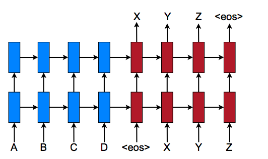
In practice, a NMT will take an input string of one language and creates a sequence of embeddings representing each element, word, in the sentence. The RNN units in the encoders take both the previous hidden state and a single element of the original input embedding as inputs, and each step can improve upon the previous step sequentially by accessing the hidden state of the previous step to inform the predicted element. It is important to also mention that in addition to encoding the sentence, an end of the sentence tag representation is included as an element in the sequence. This end of sentence tagging helps the translator know what words in the translated language will trigger the decoder to quit decoding and output the translated sentence.

The final hidden state embeddings are encoded in the intermediary encoder vector. The encodings capture as much information as possible about the input sentence in order to facilitate the decoder in decoding them into the translation. It can do this be virtue of being used as the initial hidden state for the decoder network.

Using the information from the encoder vector, each recurrent unit in the decoder accepts a hidden state from the previous unit and produces an output as well as its own hidden state. The decoder is informed by the hidden state to make a prediction on a sequence, and with each sequential prediction, it predicts the next instance of the sequence using the information from the previous hidden state. The final output is thus the end result of the step-wise predictions of each element in the translated sentence. The length of this sentence is irrelevant to the input sentences length thanks to the end of sentence tag, which tells the decoder when to stop adding terms to the sentence.

In the next section, we will show how you can implement each step using a bespoke function and PyTorch.

Implementing a Seq2Seq Translator

There is a wonderful tutorial on creating a Seq2Seq translator from scratch on the PyTorch website. This next section is adapting much of the code there, so it may be worth running through their tutorial notebook before proceeding to implement these updates.

We are going to expand upon the tutorial in two ways: adding an entirely new dataset and making tweaks to optimize the translation capability. First we will show how to acquire and prepare the WMT2014 English - French translation dataset to be used with the Seq2Seq model in a Gradient Notebook. Since much of the code is the same as in the PyTorch Tutorial, we are going to just focus on the encoder network, the attention-decoder network, and the training code.

Preparing the Data

Acquiring and Preparing the WMT2014 Europarl v7 English - French Dataset

The WMT2014 Europarl v7 English - French Dataset is a collection of speeches made within European Parliament and translated into a number of different languages. You can access it freely at https://www.statmt.org/europarl/.  

To get the dataset onto Gradient, simply go into the terminal and run

wget https://www.statmt.org/europarl/v7/fr-en.tgz
tar -xf fre-en.tgz

You will also want to download the tutorial dataset provided by Torch.

wget https://download.pytorch.org/tutorial/data.zip
unzip data.zip

Once you have the datasets, we can use some code created by Jason Brownlee from Machine Learning Mastery to quickly prepare and combine them for our NMT. This code is in the notebook data_processing.ipynb:

# load doc into memory
def load_doc(filename):
	# open the file as read only
	file = open(filename, mode='rt', encoding='utf-8')
	# read all text
	text = file.read()
	# close the file
	file.close()
	return text

# split a loaded document into sentences
def to_sentences(doc):
	return doc.strip().split('\n')

# clean a list of lines
def clean_lines(lines):
	cleaned = list()
	# prepare regex for char filtering
	re_print = re.compile('[^%s]' % re.escape(string.printable))
	# prepare translation table for removing punctuation
	table = str.maketrans('', '', string.punctuation)
	for line in lines:
		# normalize unicode characters
		line = normalize('NFD', line).encode('ascii', 'ignore')
		line = line.decode('UTF-8')
		# tokenize on white space
		line = line.split()
		# convert to lower case
		line = [word.lower() for word in line]
		# remove punctuation from each token
		line = [word.translate(table) for word in line]
		# remove non-printable chars form each token
		line = [re_print.sub('', w) for w in line]
		# remove tokens with numbers in them
		line = [word for word in line if word.isalpha()]
		# store as string
		cleaned.append(' '.join(line))
	return cleaned

# save a list of clean sentences to file
def save_clean_sentences(sentences, filename):
	dump(sentences, open(filename, 'wb'))
	print('Saved: %s' % filename)

# load English data
filename = 'europarl-v7.fr-en.en'
doc = load_doc(filename)
sentences = to_sentences(doc)
sentences = clean_lines(sentences)
save_clean_sentences(sentences, 'english.pkl')
# spot check
for i in range(10):
	print(sentences[i])

# load French data
filename = 'europarl-v7.fr-en.fr'
doc = load_doc(filename)
sentences = to_sentences(doc)
sentences = clean_lines(sentences)
save_clean_sentences(sentences, 'french.pkl')
# spot check
for i in range(1):
	print(sentences[i])

This will take our WMT2014 datasets and clean them of any punctuation, uppercase letters, non-printable characters, and tokens with numbers in them. Then it pickles the files for later use.

with open('french.pkl', 'rb') as f:
    fr_voc = pickle.load(f)

with open('english.pkl', 'rb') as f:
    eng_voc = pickle.load(f)
    
data = pd.DataFrame(zip(eng_voc, fr_voc), columns = ['English', 'French'])
data

We can use pickle.load() to load in the now saved files, and then we can use the convenient Pandas DataFrame to combine the two files.

Combining our Two Datasets

In the interest of creating a fuller dataset for the translator, let's combine the two we now have.

data2 = pd.read_csv('eng-fra.txt', '\t', names = ['English', 'French'])

We need to load up the original dataset from the canonical PyTorch tutorial. With the two dataframes, we can now concatenate them and save them back in the original format used by the sample dataset from PyTorch.

data = pd.concat([data,data2], ignore_index= True, axis = 0)

data.to_csv('eng-fra.txt')

Now, our dataset can be applied to our code just like the canonical PyTorch tutorial! But first, let's look at the steps it takes to prep the dataset and see what improvements we can make. Open up the notebook seq2seq_translation_combo.ipynb and run the first cells to make sure matplotlib inline is working and the imports are done.

from __future__ import unicode_literals, print_function, division
from io import open
import unicodedata
import string
import re
import random

import torch
import torch.nn as nn
from torch import optim
import torch.nn.functional as F

import torchtext
from torchtext.data import get_tokenizer

device = torch.device("cuda" if torch.cuda.is_available() else "cpu")

Dataset Preparation Helper Functions

SOS_token = 0
EOS_token = 1


class Lang:
    def __init__(self, name):
        self.name = name
        self.word2index = {}
        self.word2count = {}
        self.index2word = {0: "SOS", 1: "EOS"}
        self.n_words = 2  # Count SOS and EOS

    def addSentence(self, sentence):
        for word in sentence.split(' '):
            self.addWord(word)

    def addWord(self, word):
        if word not in self.word2index:
            self.word2index[word] = self.n_words
            self.word2count[word] = 1
            self.index2word[self.n_words] = word
            self.n_words += 1
        else:
            self.word2count[word] += 1

To process our dataset for the translator, we can use this Lang class to provide helpful functionality to our language class, like word2index, index2word, and word2count. The next cell will contain useful functions for cleaning the original dataset as well.

def readLangs(lang1, lang2, reverse=False):
    print("Reading lines...")

    # Read the file and split into lines
    lines = open('%s-%s2.txt' % (lang1, lang2), encoding='utf-8').\
        read().strip().split('\n')
    # Split every line into pairs and normalize
    pairs = [[normalizeString(s) for s in l.split('\t')] for l in lines]


    # Reverse pairs, make Lang instances
    if reverse:
        pairs = [list(reversed(p)) for p in pairs]
        input_lang = Lang(lang2)
        output_lang = Lang(lang1)
    else:
        input_lang = Lang(lang1)
        output_lang = Lang(lang2)

    return input_lang, output_lang, pairs

Next, the readLangs function takes in our csv to create input_lang, output_lang, and pairs variables that we will use to prepare our dataset. This function uses the helper functions to clean the text and normalize the strings.

MAX_LENGTH = 12

eng_prefixes = [
    "i am ", "i m ",
    "he is", "he s ",
    "she is", "she s ",
    "you are", "you re ",
    "we are", "we re ",
    "they are", "they re ", "I don t", "Do you", "I want", "Are you", "I have", "I think",
       "I can t", "I was", "He is", "I m not", "This is", "I just", "I didn t",
       "I am", "I thought", "I know", "Tom is", "I had", "Did you", "Have you",
       "Can you", "He was", "You don t", "I d like", "It was", "You should",
       "Would you", "I like", "It is", "She is", "You can t", "He has",
       "What do", "If you", "I need", "No one", "You are", "You have",
       "I feel", "I really", "Why don t", "I hope", "I will", "We have",
       "You re not", "You re very", "She was", "I love", "You must", "I can"]
eng_prefixes = (map(lambda x: x.lower(), eng_prefixes))
eng_prefixes = set(eng_prefixes)

def filterPair(p):
    return len(p[0].split(' ')) < MAX_LENGTH and \
        len(p[1].split(' ')) < MAX_LENGTH and \
        p[1].startswith(eng_prefixes)


def filterPairs(pairs):
    return [pair for pair in pairs if filterPair(pair)]
eng_prefixes

In another change from the Torch tutorial, I've extended the list of english prefixes to include the most common starting prefixes for the now combined dataset. I've also extended the max_length to 12 in an effort to create a more robust set of data points, but this likely introduces as many confounding as helpful factors. Try lowering the max_length down back to 10 and seeing how the performance changes.

def prepareData(lang1, lang2,reverse = False):
    input_lang, output_lang, pairs = readLangs(lang1, lang2, reverse)
    print("Read %s sentence pairs" % len(pairs))
    pairs = filterPairs(pairs)
    print("Trimmed to %s sentence pairs" % len(pairs))
    print("Counting words...")
    for pair in pairs:
        input_lang.addSentence(pair[0])
        output_lang.addSentence(pair[1])
    print("Counted words:")
    print(input_lang.name, input_lang.n_words)
    print(output_lang.name, output_lang.n_words)
    return input_lang, output_lang, pairs


input_lang, output_lang, pairs = prepareData('eng', 'fra', True)
print(random.choice(pairs))

Finally, the prepareData function puts all of the helper functions together to filter down and finalize the language pairs for NMT training. Now that our dataset is ready to go, let's jump into the code for the translator itself.

The Translator

The Encoder

class EncoderRNN(nn.Module):
    def __init__(self, input_size, hidden_size):
        super(EncoderRNN, self).__init__()
        self.hidden_size = hidden_size

        self.embedding = nn.Embedding(input_size, hidden_size)
        self.gru = nn.GRU(hidden_size, hidden_size)

    def forward(self, input, hidden):
        embedded = self.embedding(input).view(1, 1, -1)
        output = embedded
        output, hidden = self.gru(output, hidden)
        return output, hidden

    def initHidden(self):
        return torch.zeros(1, 1, self.hidden_size, device=device)

The encoder we are using is essentially the same as the tutorial, and is probably the simplest bit of code we are going to dissect in this article. We can see from the forward function how, for each input element, the encoder outputs both an output vector and a hidden state. That hidden state is then returned, so it can be used in the following step, along with the output.

The Attention-Decoder

class AttnDecoderRNN(nn.Module):
    def __init__(self, hidden_size, output_size, dropout_p=0.1, max_length=MAX_LENGTH):
        super(AttnDecoderRNN, self).__init__()
        self.hidden_size = hidden_size
        self.output_size = output_size
        self.dropout_p = dropout_p
        self.max_length = max_length

        self.embedding = nn.Embedding(self.output_size, self.hidden_size)
        self.attn = nn.Linear(self.hidden_size * 2, self.max_length)
        self.attn_combine = nn.Linear(self.hidden_size * 2, self.hidden_size)
        self.dropout = nn.Dropout(self.dropout_p)
        self.gru = nn.GRU(self.hidden_size, self.hidden_size)
        self.out = nn.Linear(self.hidden_size, self.output_size)

    def forward(self, input, hidden, encoder_outputs):
        embedded = self.embedding(input).view(1, 1, -1)
        embedded = self.dropout(embedded)

        attn_weights = F.softmax(
            self.attn(torch.cat((embedded[0], hidden[0]), 1)), dim=1)
        attn_applied = torch.bmm(attn_weights.unsqueeze(0),
                                 encoder_outputs.unsqueeze(0))

        output = torch.cat((embedded[0], attn_applied[0]), 1)
        output = self.attn_combine(output).unsqueeze(0)

        output = F.relu(output)
        output, hidden = self.gru(output, hidden)

        output = F.log_softmax(self.out(output[0]), dim=1)
        return output, hidden, attn_weights

    def initHidden(self):
        return torch.zeros(1, 1, self.hidden_size, device=device)

Since we are using attention in the example, let's look at how we can implement it in our decoder. As is immediately apparent, there are some key differences here between the encoder and decoder networks, far beyond being a simple inversion of their behaviors.

First, there are an additional 2 parameters for the init() function: max_length and dropout_p. max_length is the maximum number of elements a sentence can hold to be considered. We set this due to the large variation in sentence lengths in the two paired datasets. dropout_p  is used to aid with regularization and preventing the co-adaptation of neurons.

Second, we have the attention layer itself. At each step, the attention layer receives attention input, a decoder state, and all encoder states. It uses this to compute attention scores. For each encoder state, attention computes its "relevance" for this decoder state. It applies an attention function which receives one decoder state and one encoder state and returns a scalar value. The attention scores are used to computes attention weights. These weights are a probability distribution created by applying softmax to attention scores. Finally, it computes attention output as the weighted sum of encoder states with attention weights. (1)

These additional parameters and attention mechanism enable to decoder to require far less training and overall information to develop an understanding of the relationship of all the words in the sequence.

Training

teacher_forcing_ratio = 0.5


def train(input_tensor, target_tensor, encoder, decoder, encoder_optimizer, decoder_optimizer, criterion, max_length=MAX_LENGTH):
    encoder_hidden = encoder.initHidden()

    encoder_optimizer.zero_grad()
    decoder_optimizer.zero_grad()

    input_length = input_tensor.size(0)
    target_length = target_tensor.size(0)

    encoder_outputs = torch.zeros(max_length, encoder.hidden_size, device=device)

    loss = 0

    for ei in range(input_length):
        encoder_output, encoder_hidden = encoder(
            input_tensor[ei], encoder_hidden)
        encoder_outputs[ei] = encoder_output[0, 0]

    decoder_input = torch.tensor([[SOS_token]], device=device)

    decoder_hidden = encoder_hidden

    use_teacher_forcing = True if random.random() < teacher_forcing_ratio else False

    if use_teacher_forcing:
        # Teacher forcing: Feed the target as the next input
        for di in range(target_length):
            decoder_output, decoder_hidden, decoder_attention = decoder(
                decoder_input, decoder_hidden, encoder_outputs)
            loss += criterion(decoder_output, target_tensor[di])
            decoder_input = target_tensor[di]  # Teacher forcing

    else:
        # Without teacher forcing: use its own predictions as the next input
        for di in range(target_length):
            decoder_output, decoder_hidden, decoder_attention = decoder(
                decoder_input, decoder_hidden, encoder_outputs)
            topv, topi = decoder_output.topk(1)
            decoder_input = topi.squeeze().detach()  # detach from history as input

            loss += criterion(decoder_output, target_tensor[di])
            if decoder_input.item() == EOS_token:
                break

    loss.backward()

    encoder_optimizer.step()
    decoder_optimizer.step()

    return loss.item() / target_length

The train function we are using takes in several parameters. The input_tensor and the target_tensor are the 0th and 1st index of the sentence pair respectively. The encoder is the encoder described above. The decoder is the attention decoder described above. We are switching the encoder and decoder optimizers from Stochastic Gradient Descent to Adagrad, as we found the translations to have lower loss when using Adagrad. Finally, we are using Cross Entropy Loss as our criterion, as opposed to the tutorial which used nn.NLLLoss().

We should also look at the teacher forcing ratio. This value, which is set to .5, is used to help improve the efficacy of the model. At .5,  it randomly determines whether or not to feed the target as the next input to the decoder or to use the decoders own prediction. This can help the translation converge more quickly, but may also lead to instability. For example, over using teacher enforcing could create a model with outputs with accurate grammar but no translational relation to the input.  

def trainIters(encoder, decoder, n_iters, print_every=1000, plot_every=100):
    start = time.time()
    plot_losses = []
    print_loss_total = 0  # Reset every print_every
    plot_loss_total = 0  # Reset every plot_every

    encoder_optimizer = optim.Adagrad(encoder.parameters())
    decoder_optimizer = optim.Adagrad(decoder.parameters())
    training_pairs = [tensorsFromPair(random.choice(pairs))
                      for i in range(n_iters)]
    criterion = nn.CrossEntropyLoss()

    for iter in range(1, n_iters + 1):
        training_pair = training_pairs[iter - 1]
        input_tensor = training_pair[0]
        target_tensor = training_pair[1]

        loss = train(input_tensor, target_tensor, encoder,
                     decoder, encoder_optimizer, decoder_optimizer, criterion)
        print_loss_total += loss
        plot_loss_total += loss

        if iter % print_every == 0:
            print_loss_avg = print_loss_total / print_every
            print_loss_total = 0
            print('%s (%d %d%%) %.4f' % (timeSince(start, iter / n_iters),
                                         iter, iter / n_iters * 100, print_loss_avg))

        if iter % plot_every == 0:
            plot_loss_avg = plot_loss_total / plot_every
            plot_losses.append(plot_loss_avg)
            plot_loss_total = 0

    showPlot(plot_losses)

TrainIters actually implements the training process. For the preset number of iterations, it will compute the loss. The function goes on to save the loss values so that they can be usefully plotted after training is complete.

For a deeper look at the code that goes into this translator, make sure to check out the Gradient Notebook demo containing all of this information as well as the Github page.

The Translation

hidden_size = 256
encoder = EncoderRNN(input_lang.n_words, hidden_size).to(device)
attn_decoder = AttnDecoderRNN(hidden_size, output_lang.n_words, dropout_p=0.1).to(device)

trainIters(encoder1, attn_decoder1, 75000, print_every=5000)

Now that we have set up our translator, all we need to do is instantiate our encoder and attention decoder models for training and execute the trainIters function. Make sure you run all the cells in the notebook prior to the train cell to enable the helper functions.

We are going to use a hidden size of 256, and make sure that you have your device set to device(type='cuda'). This will ensure that the RNN trains using the GPU.

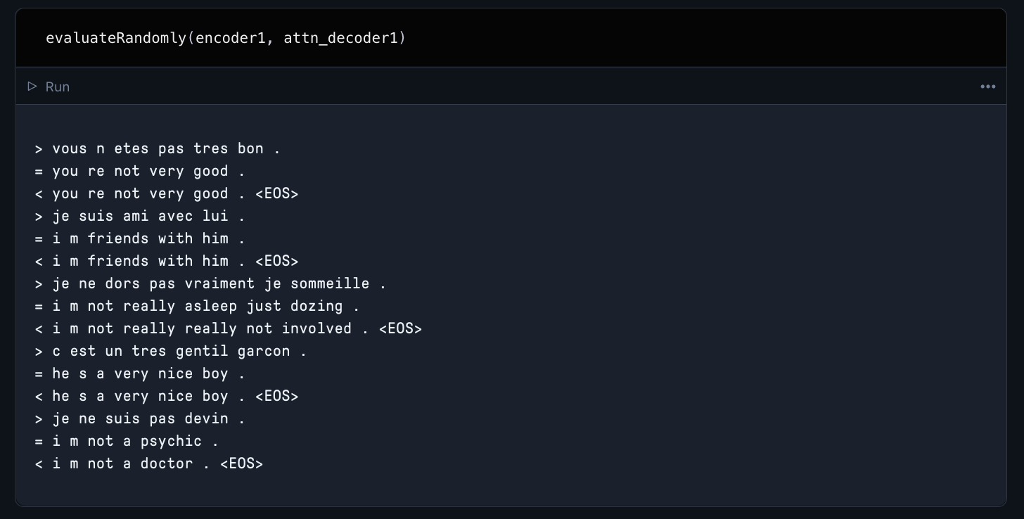
When you run this cell, your model will train for 75,000 iterations. Once training is complete, use the provided evaluation functions to assess the qualitative performance of your new translator model. Here is an example of how a model we trained for the demo performed on a random sampling of translations.

Closing thoughts

You should now be able to take any proper translation dataset and plug it into this translator code. I recommend starting with one of the other WMT Europarl pairings, but there are infinite options. Be sure to run this on Gradient to get access to a powerful GPU!

If you clone the Github repo or use it as the workspace URL in Gradient, you can access the notebooks containing the code for this article. There are three notebooks. Data processing is the notebook you should enter and run first. Then the code featured in this article for implementing Seq2Seq translation on the Europarl French-English dataset,