One application that has really caught the attention of many folks in the space of artificial intelligence is image captioning. If you think about it, there is seemingly no way to tell a bunch of numbers to come up with a caption for an image that accurately describes it. Now, with the power of deep learning, we can achieve this more accurately than we ever imagined.
The problem of writing captions for an image is two-fold: you need to get meaning out of the image by extracting relevant features, and you need to translate these features into a human-readable format. In this tutorial, we're going to look at both phases independently and then connect the pieces together. We'll start with the feature extraction phase.
This tutorial was inspired by the TensorFlow tutorial on image captioning. For this tutorial we are going to use the COCO dataset (Common Ojects in Context), which consists of over 200k labelled images, each paired with five captions.
You can run the code for this tutorial using a free GPU and Jupyter notebook on the ML Showcase.
Launch Project For Free
Step 1: Image Feature Extraction
For a given image there is always the possibility that there exist redundant elements which barely describe the image in any way. For instance, a watermark on an image of a horse race tells us virtually nothing about the image itself. We need an algorithm that can extract useful features and leave out the redundant ones, like the watermark in this case. Some years ago I probably wouldn't even be writing this tutorial because the methods used for feature extraction required a lot of math and domain-specific expertise. With the emergence of deep learning approaches, feature extraction can now be performed with minimal effort and time, meanwhile achieving more robustness with just a single neural network that has been trained on many images.
But wait, how do we obtain such a vast amount of images to cook up an incredible neural network-based feature extractor? Thanks to transfer learning, or the ability to use pre-trained models for inference on new and different problems, we don't need a single image to get started. There are many canonical convolutional network models out there that have been trained on millions of images, like ImageNet. All we need to do is slice off the task-specific part of these networks and Bob's your uncle, we have a very robust feature extractor.
When we actually dig deeper into the layers of these networks, we observe that each layer is somehow tasked during training to extract specific features. We therefore have a stack of feature extractors in one network. In this tutorial we're going to use Inception v3, a powerful model developed by Google, as our feature extractor. We can obtain this model with just three lines of Keras code.
image_model = tf.keras.applications.InceptionV3(include_top=False,
                                                weights='imagenet')
new_input = image_model.input
hidden_layer = image_model.layers[-1].output
Since each image is going to have a unique feature representation regardless of the epoch or iteration, it's recommended to run all the images through the feature extractor once and cache the extracted features on disk. This saves a lot of time since we would not need to perform forward propagation through the feature extractor during each epoch. A summarized workflow of the feature extraction process is as follows:
- Obtain the feature extraction model (in this case, we're using Inception V3)
- Use
tf.datato load an image dataset - Cache all features which are obtained from passing all images through the feature extractor once
In code, this looks like:
def load_image(image_path):
    img = tf.io.read_file(image_path)
    img = tf.image.decode_jpeg(img, channels=3)
    img = tf.image.resize(img, (299, 299))
    img = tf.keras.applications.inception_v3.preprocess_input(img)
    return img, image_path


encode_train = sorted(set(img_name_vector))

# use the tf.data api to load image dataset from directory into batches
image_dataset = tf.data.Dataset.from_tensor_slices(encode_train)
image_dataset = image_dataset.map(
  load_image, num_parallel_calls=tf.data.experimental.AUTOTUNE).batch(16)

# iterate through batches of image dataset and extract features using our feature extractor(image_features_extract_model) by doing a forward propagation.
# this is going to take some time
for img, path in image_dataset:
  batch_features = image_features_extract_model(img)
  batch_features = tf.reshape(batch_features,
                              (batch_features.shape[0], -1, batch_features.shape[3]))

# iterate through batches of features obtained from feature extractor and store in a serialized format.
for bf, p in zip(batch_features, path):
    path_of_feature = p.numpy().decode("utf-8")
    np.save(path_of_feature, bf.numpy())
Now that we're done with the first phase of our captioning task we move onto phase two, where we deal with text. This phase also uses a neural network, specifically a Recurrent Neural Network (RNN) retrofitted with some mechanisms to increase robustness to translating features to language.
Step 2: Decoding Stage
NLP
I must confess that this is the most tedious part, but we're going to keep it simple and straightforward. The first thing we're going to do here is to process our text dataset in four simple steps:
- Trim and simplify the dataset
- Tokenize the text data
- Pad sequences of words
- Batch the dataset using the
tf.dataAPI and split it into training and validation sets
Let’s see the code to do this.
Note: read the comments in the code for an explanation of each line.
top_k = 5000

# Create a tokenizer object from keras
tokenizer = tf.keras.preprocessing.text.Tokenizer(num_words=top_k,
                                                  oov_token="<unk>",
                                                  filters='!"#$%&()*+.,-/:;=?@[\]^_`{|}~ ')
# Creates a vocabulary with words from the caption dataset
tokenizer.fit_on_texts(train_captions)

# Convert each word into a unique integer
train_seqs = tokenizer.texts_to_sequences(train_captions)

# Assign token for pad
tokenizer.word_index['<pad>'] = 0
tokenizer.index_word[0] = '<pad>'

# Pads sentences. How? It calcuates the length of the longest sentence and fills the deficit of the other shorter sentences with zeros. This is to make batching possible.
cap_vector = tf.keras.preprocessing.sequence.pad_sequences(train_seqs, padding='post')

# Split each dataset into training and validation sets. Note that we're splitting both the image dataset and caption dataset.
# An image in image_name_train will correspond to its caption in cap_train.
img_name_train, img_name_val, cap_train, cap_val = train_test_split(img_name_vector,
                                                                    cap_vector,
                                                                    test_size=0.2,
                                                                    random_state=0)
dataset = tf.data.Dataset.from_tensor_slices((img_name_train, cap_train))

# Load the serialized numpy files that we stored on disk earlier
def map_func(img_name, cap):
    img_tensor = np.load(img_name.decode('utf-8')+'.npy')
    return img_tensor, cap

# Use map to load the numpy files in parallel
dataset = dataset.map(lambda item1, item2: tf.numpy_function(
          map_func, [item1, item2], [tf.float32, tf.int32]),
          num_parallel_calls=tf.data.experimental.AUTOTUNE)
BATCH_SIZE = 64
BUFFER_SIZE = 1000

# Shuffle and batch
dataset = dataset.shuffle(BUFFER_SIZE).batch(BATCH_SIZE)

# Prefetching ensures that resources don't go idle during training process. To put this another way, while the model is executing time step t, the input pipeline is loading data for time step t+1.
dataset = dataset.prefetch(buffer_size=tf.data.experimental.AUTOTUNE)
Now that we have our dataset all set up let’s go ahead and build our second network, a language model. Earlier I mentioned that our model is going to be enhanced with an attention mechanism. That’s what we'll build now.
Attention Mechanism
The whole concept of the attention mechanism is really intuitive. One popular field where the attention mechanism has become really prevalent is Neural Machine Translation, and the idea behind the attention mechanism in Machine Translation is quite similar to that in image captioning. In Machine Translation we try to translate a sentence from one language to another, and when decoding a single word (in the output sentence) we want to be "paying attention" to some specific words in the input sentence which are semantically related to that single word we are decoding.

If you want to learn more about how the attention mechanism works, or if you have any difficulty understanding the code below, check out my previous post on Neural Machine Translation.
# Bahdanau is one variant of the attention mechanism.
# The other variant is the Luong attention.

class BahdanauAttention(tf.keras.Model):
  def __init__(self, units):
    super(BahdanauAttention, self).__init__()
    self.W1 = tf.keras.layers.Dense(units)
    self.W2 = tf.keras.layers.Dense(units)
    self.V = tf.keras.layers.Dense(1)

  def call(self, features, hidden):
    # features(CNN_encoder output) shape == (batch_size, 64, embedding_dim)

    # hidden shape == (batch_size, hidden_size)
    # hidden_with_time_axis shape == (batch_size, 1, hidden_size)
    hidden_with_time_axis = tf.expand_dims(hidden, 1)

    # score shape == (batch_size, 64, hidden_size)
    score = tf.nn.tanh(self.W1(features) + self.W2(hidden_with_time_axis))
                      (batch_size,64,hidden_size) + (batch_size,1,hidden_size)
    # attention_weights shape == (batch_size, 64, 1)
    # You get 1 at the last axis because you are applying score to self.V
    attention_weights = tf.nn.softmax(self.V(score), axis=1)

    # context_vector shape after sum == (batch_size, hidden_size)
    context_vector = attention_weights * features
    context_vector = tf.reduce_sum(context_vector, axis=1)

    return context_vector, attention_weights
Recall that the output from our feature extractor is of shape batch_size*8*8*2048 (this is the shape of the output from the last layer of the Inception network immediately before the classification layer). We want to collapse this into a [batch_size*64*2048] (8*8=64) feature tensor and pass it through a single layer linear network with a ReLU activation function. This should output a tensor of shape batch_size*64*embedding_size, where the embedding size is an arbitrary integer that we set (but be sure to keep it low). The output of the linear layer is what we feed into our recurrent network retrofitted with the attention mechanism.
class CNN_Encoder(tf.keras.Model):
    def __init__(self, embedding_dim):
        super(CNN_Encoder, self).__init__()
        # shape after fc == (batch_size, 64, embedding_dim)
        self.fc = tf.keras.layers.Dense(embedding_dim)

    def call(self, x):
        x = self.fc(x)
        x = tf.nn.relu(x)
        return x
Let's finally integrate our attention network with our recurrent network.
class RNN_Decoder(tf.keras.Model):
  def __init__(self, embedding_dim, units, vocab_size):
    super(RNN_Decoder, self).__init__()
    self.units = units

    self.embedding = tf.keras.layers.Embedding(vocab_size, embedding_dim)
    self.gru = tf.keras.layers.GRU(self.units,
                                   return_sequences=True,
                                   return_state=True,
                                   recurrent_initializer='glorot_uniform')
    self.fc1 = tf.keras.layers.Dense(self.units)
    self.fc2 = tf.keras.layers.Dense(vocab_size)

    self.attention = BahdanauAttention(self.units)

  def call(self, x, features, hidden):
    # defining attention as a separate model
    context_vector, attention_weights = self.attention(features, hidden)

    # x shape after passing through embedding == (batch_size, 1, embedding_dim)
    x = self.embedding(x)

    # x shape after concatenation == (batch_size, 1, embedding_dim + hidden_size)
    x = tf.concat([tf.expand_dims(context_vector, 1), x], axis=-1)

    # passing the concatenated vector to the GRU
    output, state = self.gru(x)

    # shape == (batch_size, max_length, hidden_size)
    x = self.fc1(output)

    # x shape == (batch_size * max_length, hidden_size)
    x = tf.reshape(x, (-1, x.shape[2]))

    # output shape == (batch_size * max_length, vocab)
    x = self.fc2(x)

    return x, state, attention_weights

  def reset_state(self, batch_size):
    return tf.zeros((batch_size, self.units))


encoder = CNN_Encoder(embedding_dim)
decoder = RNN_Decoder(embedding_dim, units, vocab_size)
Now that we have a complete model, the remaining steps are the usual machine learning training and validation steps. I'll assume you're familiar with model training and gradient descent (if not, check out this post) so from here I'll dive into the validation stage.
Validation
Unlike with other machine learning validation pipelines, in this case we're not going to validate our model against a certain metric. Instead, we're going to validate our model based on whether it's generating the correct captions and, most importantly, whether it's paying attention to the correct features when generating those captions. We can achieve this by overlaying the attention matrix weights generated when producing the caption for a particular image on the image itself. This produces an image with some spots which indicate what the network was paying attention to when generating the caption. Let's look at some examples.
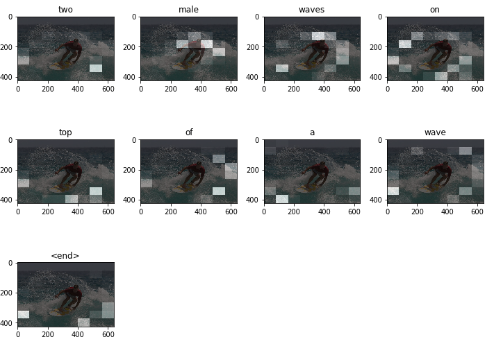
Pay close attention to the image with "male" above it. You can clearly see that most of the white boxes are clustered on the man on the surfboard with different intensities. These white boxes are an indication that the network is paying attention those regions in the image; the greater the intensity, the more attention the network is paying to that area. Decoding the captions uses a greedy search algorithm, shown in the code below. This works by feeding the decoded word at a particular time step as input to the next time step. Further improvement in decoding captions can be introduced by using a beam search decoder which is more robust than the greedy search algorithm, but a bit more complicated to implement. The code for displaying images with overlaid attention weights is also included below.
def evaluate(image):
    attention_plot = np.zeros((max_length, attention_features_shape))

    hidden = decoder.reset_state(batch_size=1)

    temp_input = tf.expand_dims(load_image(image)[0], 0)
    img_tensor_val = image_features_extract_model(temp_input)
    img_tensor_val = tf.reshape(img_tensor_val, (img_tensor_val.shape[0], -1, img_tensor_val.shape[3]))

    features = encoder(img_tensor_val)

    dec_input = tf.expand_dims([tokenizer.word_index['<start>']], 0)
    result = []

    for i in range(max_length):
        predictions, hidden, attention_weights = decoder(dec_input, features, hidden)

        attention_plot[i] = tf.reshape(attention_weights, (-1, )).numpy()

        predicted_id = tf.random.categorical(predictions, 1)[0][0].numpy()
        result.append(tokenizer.index_word[predicted_id])

        if tokenizer.index_word[predicted_id] == '<end>':
            return result, attention_plot

        dec_input = tf.expand_dims([predicted_id], 0)

    attention_plot = attention_plot[:len(result), :]
    return result, attention_plot

def plot_attention(image, result, attention_plot):
    temp_image = np.array(Image.open(image))

    fig = plt.figure(figsize=(10, 10))

    len_result = len(result)
    for l in range(len_result):
        temp_att = np.resize(attention_plot[l], (8, 8))
        ax = fig.add_subplot(len_result//2, len_result//2, l+1)
        ax.set_title(result[l])
        img = ax.imshow(temp_image)
        ax.imshow(temp_att, cmap='gray', alpha=0.6, extent=img.get_extent())

    plt.tight_layout()
    plt.show()
That's a wrap for this tutorial.
Next Steps
- Try out your model on a different dataset, like the Flickr dataset.
- Extend your knowledge into a different domain, like Neural Machine Translation. You can check out my tutorial for that here.
- Try out a different architecture, like the transformer network, which also uses attention (self-attention in this case).

