Computer vision is a popular domain, it is very known for its fast development and expansion. Over the past few years, new state-of-the-art libraries continue to be released, and it is the gateway into deep learning for many great data scientists. One of the most popular types of computer vision is image segmentation.

In this article, we will define image segmentation and Segmentation_models_PyTorch, discover the right metrics to use in these tasks, and demonstrate an end-to-end pipeline that can be used as a template for handling image segmentation problems. We will walk through the necessary steps, from data preparation to model setup using the Segmentation_models_pytorch package, which will make our task easier, to visualization of  results. Lastly, we will talk about some useful applications of image segmentation. Apart from being cool and informative.

Image segmentation:

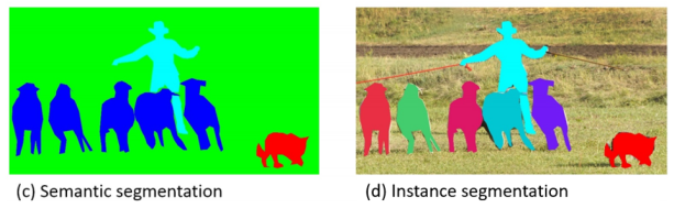
We can consider image segmentation as a classification task at the pixel level where we classify each pixel in an image, assigning it to a corresponding class, so if we have a 256*192 image, we actually have to make 48768-pixel classifications. Depending on the task, we can have a semantic segmentation where we have to classify every pixel in a photo or an instance segmentation where we only have to classify the pixels representing objects of a certain type of interest.

Metrics for image segmentation

The easiest metric to use in image segmentation tasks is pixel accuracy, as is obvious in its name, it helps us to find out the precision of pixel classification. Unfortunately, we can't completely depend on it, if the relevant pixels don't take much of a picture, then the pixel accuracy is very high, thus it didn't segment anything, so it's useless in this situation.

Therefore, there are other metrics that can be used in situations like these; for example the intersection over union and the dice coefficient, we can relate of them most of the time.

Intersection over union (IoU)

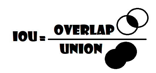
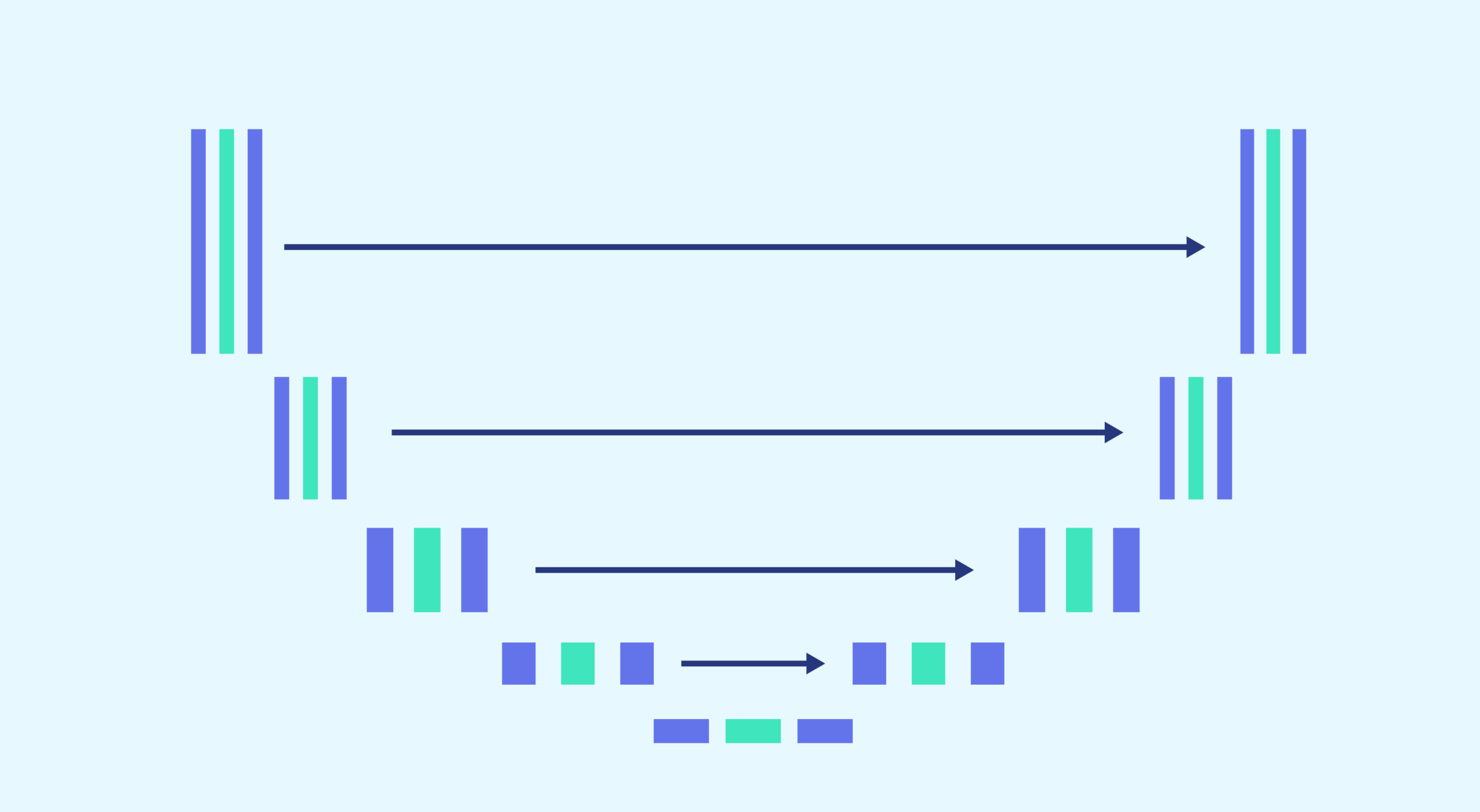
The intersection over union (IoU) is also known as the Jaccard index. Using IoU implies that we have two images to compare: one is our prediction and the other one is the ground truth, if the value obtained approaches number 1 that means the prediction is similar and close to our ground truth. And vice versa, the lower IoU, the worst our results.

In the image below, we can see a visual representation of the areas involved in the computation. We can figure out how the metric is efficiently penalized both if we predict a larger area than what it should be (the denominator will be larger) or a smaller one (the numerator will be smaller).

Dice coefficient

The other useful metric is the Dice coefficient, which is the area of overlap between the prediction and ground truth doubled and then divided by the sum of the prediction and ground truth areas:

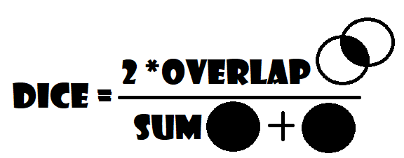
It has the same function as the last metrics, but in this one, we don't consider the union in the denominator, both are very similar, and they produce almost the same outcomes, 1 signifying the perfect match between the predicted and the truth, and the closer the value to 0, the more the prediction is afield to the wanted ground truth.

Segmentation_models_pytorch

Segmentation_models_pytorch is an awesome library built on the PyTorch framework, which is used to create a PyTorch nn.Module (with just two lines of code) for image segmentation tasks, and it contains 5 model architectures for binary and multi-class segmentation (including legendary Unet), 46 encoders for each architecture, and all encoders have pre-trained weights for faster and better convergence.

Image segmentation using segmentation_models_pytorch from scratch

In this section we will demonstrate an end-to-end pipeline that can be used as a template for handling image segmentation problems, we will use Supervise.ly Filtered Segmentation Person Dataset from Kaggle, which contains 2667 person images and their segmentation.

Let's start by loading the necessary libraries.

Load all dependencies we need

We first will import numpy for linear algebra, and os for interaction with the operating system. Then, we want to use PyTorch, so we import torch, and from there we import nn. That will help us create and train the network, and also let us import optim, a package that implements various optimization algorithms (e.g. sgd, adam,..). From torch.utils.data we import Dataset to prepare the dataset and DataLoader to create mini batch sizes.

We will import also torchvision since we are working with images, segmentation_models_pytorch to make our task easier, albumentations for data augmentation, tqdm to show progress bars, and finally matplotlib.pyplot to show the results and compare them with the ground truth.

import os
import numpy as np
from PIL import Image
import torch
from torch import nn, optim
from torch.utils.data import Dataset, DataLoader
import torchvision
import segmentation_models_pytorch as smp
import albumentations as A  
from albumentations.pytorch import ToTensorV2
from tqdm import tqdm
import matplotlib.pyplot as plt

Seed everything

Let's seed everything to make results somewhat reproducible

def seed_everything(seed):
    os.environ["PYTHONHASHSEED"] = str(seed)
    np.random.seed(seed)
    torch.manual_seed(seed)
    torch.cuda.manual_seed(seed)
    torch.backends.cudnn.deterministic = True
    torch.backends.cudnn.benchmark = True
    
seed_everything(42)

Dataset

To set up the data loading part, we are going to create a class with the name SegmentationDataset, and inherit it from Dataset. This class will have three methods:

• init: that take as parameters self, input directory that contains person images, output directory that contains person segmentation images, transform for data transformation that will be None by default, is_train which will be True while training phase with 80% of the data, and it will be False while validating phase with 20% of the data.
• len: It will return the length of the dataset.
• getitem: That takes as input self and index, and we'll get the image path which is going to be the path of the image directory where we stored the images, and join it with the file of that particular image, then we do the same to get the mask path. So now that we have the mask path and the image path, we load those two, after converting the mask into L to turn it into a grayscale (1 channel) and the image to RGB (3 channels), then convert them into NumPy arrays because we're using the albumentations library, divide them by 255  to have pixels between 0 and 1, apply transform to them if it isn't None, and finally return the image and the mask.

class SegmentationDataset(Dataset):
    def __init__(self, input_dir, output_dir, is_train, transform=None):
        self.input_dir  = input_dir
        self.output_dir = output_dir
        self.transform  = transform
        if is_train == True:
            x = round(len(os.listdir(input_dir)) * .8)
            self.images = os.listdir(input_dir)[:x]
        else:
            x = round(len(os.listdir(input_dir)) * .8)
            self.images = os.listdir(input_dir)[x:]

    def __len__(self):
        return len(self.images)

    def __getitem__(self, index):
        img_path    = os.path.join(self.input_dir, self.images[index])
        mask_path   = os.path.join(self.output_dir, self.images[index])
        img         = np.array(Image.open(img_path).convert("RGB"), dtype=np.float32) / 255
        mask        = np.array(Image.open(mask_path).convert("L"), dtype=np.float32)   / 255
        
        if self.transform is not None:
            augmentations = self.transform(image=img, mask=mask)
            img   = augmentations["image"]
            mask  = augmentations["mask"]
        
        return img, mask

Hyperparameters and Initializations

Let's initialize train_inp_dir by the path of the images, train_out_dir by the path of the masks, and device by Cuda if it is available and CPU otherwise. Set up some hyperparameters (learning rate, batch size, number of epochs...). Finally, initialize transforms for training that contains resize images and some augmentations (horizontal flip and color jitter), and convert them to tensors. It is the same process for validation, except for augmentations.

TRAIN_INP_DIR = '../input/supervisely-filtered-segmentation-person-dataset/supervisely_person_clean_2667_img/images/'
TRAIN_OUT_DIR = '../input/supervisely-filtered-segmentation-person-dataset/supervisely_person_clean_2667_img/masks/'
DEVICE        = "cuda" if torch.cuda.is_available() else "cpu"

LEARNING_RATE = 3e-4
BATCH_SIZE    = 64
NUM_EPOCHS    = 10
IMAGE_HEIGHT  = 256  
IMAGE_WIDTH   = 192  

train_transform = A.Compose(
    [
        A.Resize(height=IMAGE_HEIGHT, width=IMAGE_WIDTH),
        A.ColorJitter(p=0.2),
        A.HorizontalFlip(p=0.5),
        ToTensorV2(),
    ],
)

val_transform = A.Compose(
    [
        A.Resize(height=IMAGE_HEIGHT, width=IMAGE_WIDTH),
        ToTensorV2(),
    ],
)

Now let's create a function get_loaders that uses the SegmentationDataset class to prepare the data and DataLoader to create mini-batch sizes, in order to return train_loader and val_loader

def get_loaders( inp_dir, mask_dir,batch_size,
			     train_transform, val_tranform ):
    
    train_ds     = SegmentationDataset( input_dir=inp_dir, output_dir=mask_dir,
                            is_train=True, transform=train_transform)

    train_loader = DataLoader( train_ds, batch_size=batch_size, shuffle=True )

    val_ds       = SegmentationDataset( input_dir=inp_dir, output_dir=mask_dir,
                            is_train=False, transform=val_transform)

    val_loader   = DataLoader( val_ds, batch_size=batch_size, shuffle=True  )

    return train_loader, val_loader

Check Data loader

Let's check if everything works fine and see what the data looks like.

train_loader, val_loader = get_loaders( TRAIN_INP_DIR, TRAIN_OUT_DIR,
                            BATCH_SIZE,  train_transform, val_transform)
inputs, masks = next(iter(train_loader))

_, ax = plt.subplots(1,2)
ax[0].imshow(inputs[0].permute(1,2,0))
ax[1].imshow(masks[0])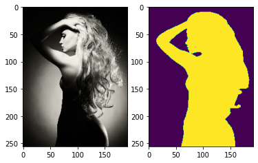

Check accuracy:

Let's build the check_accuracy function to check the validation accuracy of our model using pixel accuracy and dice score, we send to the function the loader, model, and device.

We set up num_correct, num_pixels, and dice_score to 0 to calculate pixel accuracy and dice score letter.

We switch the model to evaluation mode and wrap everything with torch.no_grad, after that we go through loader, move the image and their mask into the device, and run through the model to get some prediction using sigmoid to make the pixels between 0 and 1, then convert all those that are higher than 0.5 to 1, and all those less than that to 0,  because for segmentation we're outputting a prediction for each individual pixel  (1 for a person and 0 otherwise) then we calculate the number of correct predictions divided by the number of pixels to calculate pixel accuracy, next we calculate dice score. Finally, we switch the model to training mode.

def check_accuracy(loader, model, device="cuda"):
    num_correct = 0
    num_pixels  = 0
    dice_score  = 0
    model.eval()

    with torch.no_grad():
        for img, mask in tqdm(loader):
            img   = img.to(device)
            mask  = mask.to(device).unsqueeze(1)
            preds = torch.sigmoid(model(img))
            preds = (preds > 0.5).float()
            num_correct += (preds == mask).sum()
            num_pixels += torch.numel(preds)
            dice_score += (2 * (preds * mask).sum()) / (
                (preds + mask).sum() + 1e-7
            )

    print(
        f"Got {num_correct}/{num_pixels} with pixel accuracy {num_correct/num_pixels*100:.2f}"
    )
    print(f"Dice score: {dice_score/len(loader)*100:.2f}")
    model.train()

Model, loss function, and optimizer

In this model we will use UNet, which is a semantic segmentation technique originally proposed for medical imaging segmentation. Up to now, it has outperformed the prior best method for segmentation in general, also used in many advanced GANs such as pix2pix.

• We will build such a powerful model with just one line of code using Segmentation_models_pytorch, we chose the legendary UNet architecture with transfer learning 'efficientnet-b3', with number of input 3 (RGB), number of classes 1, without using any activation function. But before using the predictions, we use sigmoid to have the pixels between 1 and 0. lastly, we move the model to the device.
• We have a binary class segmentation, so basically, it's just a binary classification task at the pixel level, so in the loss function, we will use BCEWithLogitsLoss.
• For the optimizer, we will use Adam.

model = smp.Unet(encoder_name='efficientnet-b3', in_channels=3, classes=1, activation=None).to(DEVICE)
loss_fn   = nn.BCEWithLogitsLoss()
optimizer = optim.Adam(model.parameters(), lr=LEARNING_RATE)

Training

Now the fun part, where the magic will happen, in this section we will train our model.

• We loop for all the mini batch sizes that we create with the DataLoader, move the images and their masks into the device.
• For forward pass, we use the model to predict the masks and calculate the loss between the predictions and the ground truth.
• For the backward pass, we set the gradients to zero because otherwise the gradients are accumulated (default behavior in PyTorch), then we use the loss to backpropagate method, and we update the weights.
• Last but not least, we update tqdm loop.

def train_fn(loader, model, optimizer, loss_fn):
    loop = tqdm(loader)

    for batch_idx, (image, mask) in enumerate(loop):
        image   = image.to(device=DEVICE)
        mask    = mask.float().unsqueeze(1).to(device=DEVICE)

        # forward
        predictions = model(image)
        loss = loss_fn(predictions, mask)

        # backward
        model.zero_grad()
        loss.backward()
        optimizer.step()

        # update tqdm loop
        loop.set_postfix(loss=loss.item())

Let's check accuracy before any training for fun.

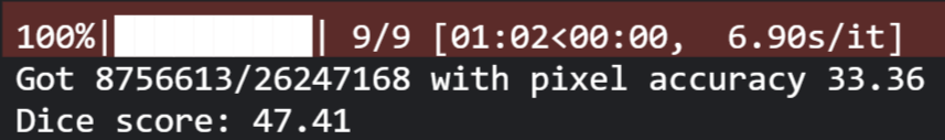
check_accuracy(val_loader, model, device=DEVICE)

Now let's move to train the model and check the accuracy after each epoch.

for epoch in range(NUM_EPOCHS):

    print('########################## epoch: '+str(epoch))
    train_fn(train_loader, model, optimizer, loss_fn)
    
    # check accuracy
    check_accuracy(val_loader, model, device=DEVICE)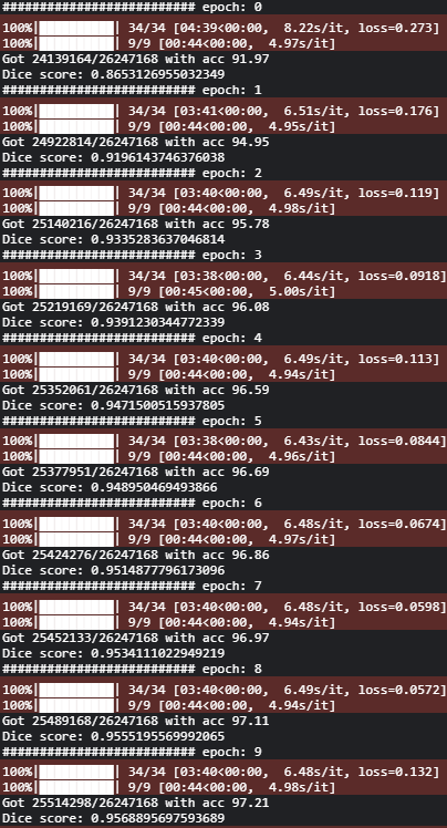

We can see that we get a pixel accuracy of 97.21% and a dice score of 95.68%.

Visualize results

Now the moment of the truth, let's visualize the results and compare them with the ground truth.

inputs, masks = next(iter(val_loader))
output        = ((torch.sigmoid(model(inputs.to('cuda')))) >0.5).float()
_, ax = plt.subplots(2,3, figsize=(15,10))
for k in range(2):
    ax[k][0].imshow(inputs[k].permute(1,2,0))
    ax[k][1].imshow(output[k][0].cpu())
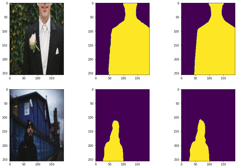
    ax[k][2].imshow(masks[k])

The image below represents the output of this code, in the first column, we find the images themselves, in the second column we have the predictions, and in the last one the ground truth.

You might not have the same image because we are shuffling the data

Applications of image segmentation

There are many useful applications of image segmentation such as:

• Medical images

image segmentation is the most useful thing, it is very essential in knowing and diagnosing the different diseases and also pattern recognition research. For example, in imaging field is used to locate tumors, study anatomical structure, etc.

• Object detection

The main role and function of image segmentation are to identify an image and analyze it, by detecting objects, understanding interactions, etc. which makes It a lot easier than finding meaning from pixels. For example, if we take a photo of a newspaper, a segmentation process can be employed to separate images and text in that newspaper. From your photo, eyes, nose or mouth can be separated from the rest of the image.

There are many other helpful applications of image segmentation like image editing, counting things in images(people in a crowd, stars in the sky...), and locating some objects in satellite images(roads, forests...).