The applications of deep learning models and computer vision in the modern era are growing by leaps and bounds. Computer vision is one such field of artificial intelligence where we train our models to interpret real-life visual images. With the help of deep learning architectures like U-Net and CANet, we can achieve high-quality results on computer vision datasets to perform complex tasks. While computer vision is a humungous field with so much to offer and so many different, unique types of problems to solve, our focus for the next couple of articles will be on two architectures, namely U-Net and CANet, that are designed to solve the task of image segmentation.
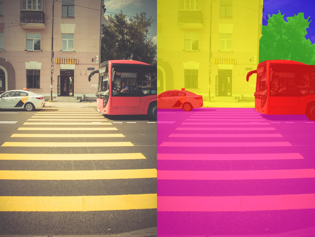
The task in image segmentation is to take an image and divide it into several smaller fragments. These fragments or these multiple segments produced will help with the computation of image segmentation tasks. For image segmentation tasks, another essential requirement is the use of masks. With the help of masking, which is basically a binary image consisting of zero or non-zero values, we can obtain the desired result required for the segmentation task. Once we describe the most essential constituents of the image obtained during image segmentation with the help of images and their respective masks, we can achieve a multitude of future tasks with them.
Some of the most crucial applications of image segmentation include machine vision, object detection, medical image segmentation, machine vision, face recognition, and so much more. Before you dive into this article, I would suggest checking out some optional pre-requisites to follow along with this article. I would recommend checking the TensorFlow and Keras guides to get familiar with these deep learning frameworks as we will utilize them to construct the U-Net architecture. Below is the list of the table of contents for understanding the list of concepts that we will cover in this article. It is recommended to follow through the entire article, but you can feel free to check out the specific sections if you know some concepts already.
Table Of Contents:
- Introduction To U-Net
- Understanding The U-Net Architecture
- TensorFlow Implementation of U-Net
1. Modifications in the implemented model
2. Importing the required libraries
3. Building the Convolution Block
4. Constructing the encoder and decoder blocks
5. Construct the U-Net architecture
6. Finalizing the model - Quick Example Project To View U-Net Performance
1. Dataset Preparation
2. Data Visualization
3. Configure the data generator
4. U-Net Model
5. Train the model
6. View the results - Conclusion
Introduction To U-Net:
The U-Net architecture, first published in the year 2015, has been a revolution in the field of deep learning. The architecture won the International Symposium on Biomedical Imaging (ISBI) cell tracking challenge of 2015 in numerous categories by a large margin. Some of their works include the segmentation of neuronal structures in electron microscopic stacks and transmitted light microscopy images.
With this U-Net architecture, the segmentation of images of sizes 512X512 can be computed with a modern GPU within small amounts of time. There have been many variants and modifications of this architecture due to its phenomenal success. Some of them include LadderNet, U-Net with attention, the recurrent and residual convolutional U-Net (R2-UNet), and U-Net with residual blocks or blocks with dense connections.
Although U-Net is a significant accomplishment in the field of deep learning, it is equally essential to understand the previous methods that were employed for solving such kind of similar tasks. One of the primary examples that comes to end was the sliding window approach, which won the EM segmentation challenge at ISBI in the year 2012 by a large margin. The sliding window approach was able to generate a wide array of sample patches apart from the original training dataset.
This result was because it used the method of setting up the network of sliding window architecture by making the class label of each pixel as separate units by providing a local region (patch) around that pixel. Another achievement of this architecture was the fact that it could localize quite easily on any giving training dataset for the respective tasks.
However, the sliding window approach suffered two main drawbacks that were countered by the U-Net architecture. Since each pixel was considered separately considered, the resulting patches we overlapping a lot. Hence, a lot of overall redundancy was produced. Another limitation was that the overall training procedure was quite slow and consumed a lot of time and resources. The feasibility of the working of the network is questionable due to the following reasons.
The U-Net is an elegant architecture that solves most of the occurring issues. It uses the concept of fully convolutional networks for this approach. The intent of the U-Net is to capture both the features of the context as well as the localization. This process is completed successfully by the type of architecture built. The main idea of the implementation is to utilize successive contracting layers, which are immediately followed by the upsampling operators for achieving higher resolution outputs on the input images.
Understanding The U-Net Architecture:
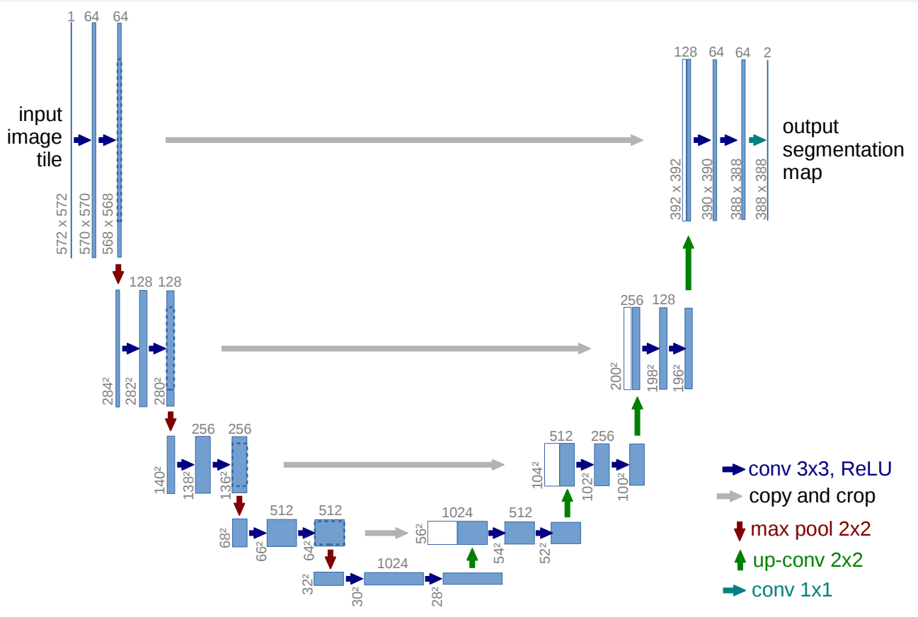
By having a brief look at the architecture shown in the image, we can notice why it is probably referred to as U-Net architecture. The shape of the so formed architecture is in the form of a 'U' and hence the following name. Just by looking at the structure and the numerous elements involved in the process of the construction of this architecture, we can understand that the network built is a fully convolutional network. They have not used any other layers such as dense or flatten or other similar layers. The visual representation shows an initial contracting path followed by an expanding path.
The architecture shows that an input image is passed through the model and then it is followed by a couple of convolutional layers with the ReLU activation function. We can notice that the image size is reducing from 572X572 to 570X570 and finally to 568X568. The reason for this reduction is because they have made use of unpadded convolutions (defined the convolutions as "valid"), which results in the reduction of the overall dimensionality. Apart from the Convolution blocks, we also notice that we have an encoder block on the left side followed by the decoder block on the right side.
The encoder block has a constant reduction of image size with the help of the max-pooling layers of strides 2. We also have repeated convolutional layers with an increasing number of filters in the encoder architecture. Once we reach the decoder aspect, we notice the number of filters in the convolutional layers start to decrease along with a gradual upsampling in the following layers all the way to the top. We also notice that the use of skip connections that connect the previous outputs with the layers in the decoder blocks.
This skip connection is a vital concept to preserve the loss from the previous layers so that they reflect stronger on the overall values. They are also scientifically proven to produce better results and lead to faster model convergence. In the final convolution block, we have a couple of convolutional layers followed by the final convolution layer. This layer has a filter of 2 with the appropriate function to display the resulting output. This final layer can be changed according to the desired purpose of the project you are trying to perform.
TensorFlow Implementation of U-Net
In this section of the article, we will look at the TensorFlow implementation of the U-Net architecture. While I am utilizing TensorFlow for computation of the model, you can choose any deep learning framework such as PyTorch for a similar implementation. We will look at the working of the U-Net architecture along with some other model structures with PyTorch in future articles. However, for this article, we will stick to the TensorFlow library. We will be importing all the required libraries and constructing our U-Net architecture from scratch. But, we will make some necessary changes that will improve the overall performance of the model as well as make it slightly less complex.
- Modifications in the implemented model
It is crucial to note that the U-Net model was introduced way back in 2015. Although its performance at that point in time was fabulous, the prominent methods and functions of deep learning have evolved simultaneously as well. Hence, there have many successful variants and versions of the U-Net architecture since its original creation to preserve certain image qualities while replicating, and in some scenarios, performing better than the original architecture.
I will try to preserve most of the essential parameters and architectural elements of the original implementation of the U-Net architecture. However, there will be slight changes from the original content that will improve the modern efficiency and improve the speed as well the simplicity of the model. One of the changes that will be included in this structure is using the value of Convolution as "same" because many pieces of research in the future have shown that this particular change did not negatively impact the architectural build in any way. Also, since the concept of batch normalization was introduced in 2016, the original architecture did not use this aspect. But, our model implementation will include batch normalization as it yields the best results in most cases.
- Importing the required libraries
For building the U-Net architecture, we will utilize the TensorFlow deep learning framework, as discussed already. Hence, we will import the TensorFlow library for this purpose as well as the Keras framework, which is now an integral part of TensorFlow model structures. From our previous understanding of the U-Net architecture, we know that some of the essential imports include the convolutional layer, the max-pooling layer, an input layer, and the activation function ReLU for the basic modeling structure. We will then use some additional layers like the Conv2DTranspose layer, which will perform an upsampling for our desired decoder blocks. We will also make use of the Batch Normalization layers for stabilizing the training process and use the Concatenate layers for combining the necessary skip connections.
import tensorflow as tf
from tensorflow import keras
from tensorflow.keras.layers import Input, Conv2D, MaxPooling2D, Activation, ReLU
from tensorflow.keras.layers import BatchNormalization, Conv2DTranspose, Concatenate
from tensorflow.keras.models import Model, Sequential- Building the Convolution Block
After importing the required libraries, we can continue to build the U-Net architecture. You can either do this in one complete class by defining all the parameters and values accordingly in order and continuing the process until you reach the very end or you a few iterative blocks. I will be using the latter method as it is more convenient for most users to understand the model architecture of U-Net with the help of few blocks. We will utilize three iterative blocks as shown in the architecture representation, namely the convolution operation block, the encoder block, and the decoder block. With the help of these three blocks, we can build the U-Net architecture with ease. Let us now process and understand each of these function code blocks one by one.
The convolution operation block is used to perform the primary operation of taking the entered input parameters and processing a double layer of convolution operations. In this function, we have two arguments, namely the input for the convolution layer and the number of filters, which is by default 64. We will use the value of padding as same as discussed previously to maintain the same shapes as opposed to unpadded or valid convolutions. These convolutional layers are followed along by the Batch Normalization layer. These changes from the original model are made to gain the best outcomes possible. Finally, a ReLU activation layer is added into the mix as defined in the research paper. Let us explore the code block for building the convolution block.
def convolution_operation(entered_input, filters=64):
    # Taking first input and implementing the first conv block
    conv1 = Conv2D(filters, kernel_size = (3,3), padding = "same")(entered_input)
    batch_norm1 = BatchNormalization()(conv1)
    act1 = ReLU()(batch_norm1)

    # Taking first input and implementing the second conv block
    conv2 = Conv2D(filters, kernel_size = (3,3), padding = "same")(act1)
    batch_norm2 = BatchNormalization()(conv2)
    act2 = ReLU()(batch_norm2)

return act2- Constructing the encoder and decoder blocks
Our Next step will be to build the encoder and decoder blocks. These two functions are quite simple to construct. The encoder architecture will use consecutive inputs starting from the first layer all the way to the bottom. The encoder function as we have defined will have the convolutional block, i.e., two convolutional layers followed by their respective batch normalization and ReLU layers. Once we pass them through the convolution blocks, we will quickly downsample these elements, as mentioned in the research paper. We will use a max-pooling layer and stick to the parameters mentioned in the paper as the strides = 2. We will then return both the initial output and the max-pooled output, as we need the former for performing the skip connections.
The decoder block will include three arguments, namely the receiving inputs, the input of the skip connection, and the number of filters in the particular building block. We will upsample the entered input with the help of the Conv2DTranspose layers in our model. We will then concatenate both the receiving input and the newly upsampled layers to receive the final value of the skip connections. We will then use this combined function and perform our convolutional block operation to proceed to the next layer and return this output value.
def encoder(entered_input, filters=64):
    # Collect the start and end of each sub-block for normal pass and skip connections
    enc1 = convolution_operation(entered_input, filters)
    MaxPool1 = MaxPooling2D(strides = (2,2))(enc1)
    return enc1, MaxPool1
def decoder(entered_input, skip, filters=64):
# Upsampling and concatenating the essential features
Upsample = Conv2DTranspose(filters, (2, 2), strides=2, padding="same")(entered_input)
Connect_Skip = Concatenate()([Upsample, skip])
out = convolution_operation(Connect_Skip, filters)
return out- Construct the U-Net architecture:
If you are trying to build the entire U-Net architecture from scratch in a single layer, you might find that the overall structure is quite humungous because it consists of so many different blocks to be processed. By dividing our respective functions into three separate code blocks of convolutional operation, encoder structure, and decoder structure, we can construct the U-Net architecture with ease in a few lines of code. We will use the input layer, which will contain the respective shapes of our input image.
After this step, we will collect all the primary outputs and the skip outputs to pass them on to further blocks. We will create the next block and construct the entire decoder architecture until we reach the output. The output will have the required dimensions according to our desired output. In this case, I have one output node with the sigmoid activation function. We will call the functional API modeling system to create our final model and return this model to the user for performing any task with the U-Net architecture.
def U_Net(Image_Size):
    # Take the image size and shape
    input1 = Input(Image_Size)

    # Construct the encoder blocks
    skip1, encoder_1 = encoder(input1, 64)
    skip2, encoder_2 = encoder(encoder_1, 64*2)
    skip3, encoder_3 = encoder(encoder_2, 64*4)
    skip4, encoder_4 = encoder(encoder_3, 64*8)

    # Preparing the next block
    conv_block = convolution_operation(encoder_4, 64*16)

    # Construct the decoder blocks
    decoder_1 = decoder(conv_block, skip4, 64*8)
    decoder_2 = decoder(decoder_1, skip3, 64*4)
    decoder_3 = decoder(decoder_2, skip2, 64*2)
    decoder_4 = decoder(decoder_3, skip1, 64)

    out = Conv2D(1, 1, padding="same", activation="sigmoid")(decoder_4)

    model = Model(input1, out)
return model- Finalizing the Model:
Ensure that your image shapes are divisible by at least 16 or multiples of 16. Since we are using four max-pooling layers during the down-sampling procedure, we don't want to encounter the divisibility of any odd number shapes. Hence, it would be best to ensure that the sizes of your architecture are equivalent to sizes like (48, 48), (80,80), (160, 160), (256, 256), (512, 512), and other similar shapes. Let us try our model structure for an input shape of (160, 160, 3) and test the results. A summary of the model and its respective plot is obtained. You can see both these structures from the attached Jupyter Notebook. I will also include the model.png to show the particular plot of the entire architectural build.
input_shape = (160, 160, 3)
model = U_Net(input_shape)
model.summary()
tf.keras.utils.plot_model(model, "model.png", show_shapes=False, show_dtype=False, show_layer_names=True, rankdir='TB', expand_nested=False, dpi=96)You can view the summary and plots respectively with the above code blocks. Let us now explore a fun project with the U-Net architecture.
Quick Example Project To View U-Net Performance:
For this project, we will use the reference from Keras for an image segmentation project. The following link will guide you to the reference. For this project, we will extract the dataset and visualize the basic elements to get an overview of the structure. We can then proceed to build the data generator for loading for data from the dataset accordingly. We will then utilize the U-Net model that we built in the previous section and train this model until we reach a satisfactory result. Once our desired result is obtained, we will save this model and test it out on a validation sample. Let us get started with the implementation of the project!
- Dataset Preparation
We will use the Oxford pet dataset for this particular task of image segmentation. The Oxford pet dataset consists of 37 categories of pet dataset with roughly 200 images for each class. The images have a large variation in scale, pose, and lighting. To install the dataset locally on your system, you can download the images dataset from this link and the annotations dataset from the following link. Once you have the zip files downloaded successfully, you can unzip them twice with 7-zip or any other similar tool kit that you use on your operating system.
In the first code block, we will define the respective paths to the images and annotations directories. We will also define some essential parameters such as the image size, the batch size, and the number of classes. We will then ensure that all the elements in the dataset are arranged in the correct order for performing and obtaining a satisfactory image segmentation task. You can verify the images with their respective annotations by printing both the file paths to check if they produce the desired results.
import os

input_dir = "images/"
target_dir = "annotations/trimaps/"
img_size = (160, 160)
num_classes = 3
batch_size = 8

input_img_paths = sorted(
    [
        os.path.join(input_dir, fname)
        for fname in os.listdir(input_dir)
        if fname.endswith(".jpg")
    ]
)
target_img_paths = sorted(
    [
        os.path.join(target_dir, fname)
        for fname in os.listdir(target_dir)
        if fname.endswith(".png") and not fname.startswith(".")
    ]
)

print("Number of samples:", len(input_img_paths))

for input_path, target_path in zip(input_img_paths[:10], target_img_paths[:10]):
print(input_path, "|", target_path)- Data Visualization
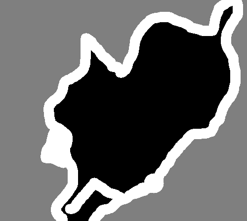
Now that we have collected and pre-processed our data for our project, our next step will be to take a brief look at the dataset. Let us analyze the dataset by displaying both an image and its respective segmented output. This segmented output with the masking is often times referred to as the ground truth annotation. We will utilize the I-Python display option along with the pillow library for randomly displaying a selected image. This simple code block is written as follows:
from IPython.display import Image, display
from tensorflow.keras.preprocessing.image import load_img
import PIL
from PIL import ImageOps

# Display input image #7
display(Image(filename=input_img_paths[9]))

# Display auto-contrast version of corresponding target (per-pixel categories)
img = PIL.ImageOps.autocontrast(load_img(target_img_paths[9]))
display(img)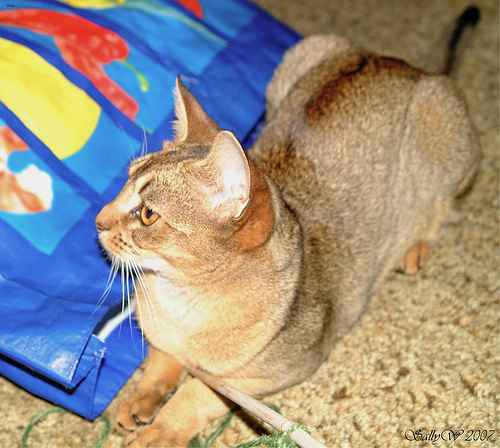
- Configure the data generator
In this particular code block, instead of using data generators to prepare the data, we will utilize the Sequence operation from the Keras deep learning framework. This method is much safer for multi-processing in comparison to using the generator because they only train each sample once per epoch, which will avoid any unnecessary adjustments that we will need to make. We will then prepare the Sequence class in the utils module of Keras to compute, load, and vectorize batches of data. We will then construct the initialization function, an additional function to compute the length and the final function that will generate batches of data.
from tensorflow import keras
import numpy as np
from tensorflow.keras.preprocessing.image import load_img


class OxfordPets(keras.utils.Sequence):
    """Helper to iterate over the data (as Numpy arrays)."""

    def __init__(self, batch_size, img_size, input_img_paths, target_img_paths):
        self.batch_size = batch_size
        self.img_size = img_size
        self.input_img_paths = input_img_paths
        self.target_img_paths = target_img_paths

    def __len__(self):
        return len(self.target_img_paths) // self.batch_size

    def __getitem__(self, idx):
        """Returns tuple (input, target) correspond to batch #idx."""
        i = idx * self.batch_size
        batch_input_img_paths = self.input_img_paths[i : i + self.batch_size]
        batch_target_img_paths = self.target_img_paths[i : i + self.batch_size]
        x = np.zeros((self.batch_size,) + self.img_size + (3,), dtype="float32")
        for j, path in enumerate(batch_input_img_paths):
            img = load_img(path, target_size=self.img_size)
            x[j] = img
        y = np.zeros((self.batch_size,) + self.img_size + (1,), dtype="uint8")
        for j, path in enumerate(batch_target_img_paths):
            img = load_img(path, target_size=self.img_size, color_mode="grayscale")
            y[j] = np.expand_dims(img, 2)
            # Ground truth labels are 1, 2, 3. Subtract one to make them 0, 1, 2:
            y[j] -= 1
        return x, y
In the next step, we will define the split between the training and the validation data, respectively. We do this step to ensure that there is no corruption between the integrity of the elements in the train and test sets accordingly. Both of these data entities must be viewed separately so that the model does not get a peek at the testing data. In the validation set, we will also perform an optional shuffle operation that will mix up all the images in the dataset, and we can obtain random samples for both the train and the validation images. We will then call the training values and the validation values individually and store them in their respective variables.
import random

# Split our img paths into a training and a validation set
val_samples = 1000
random.Random(1337).shuffle(input_img_paths)
random.Random(1337).shuffle(target_img_paths)
train_input_img_paths = input_img_paths[:-val_samples]
train_target_img_paths = target_img_paths[:-val_samples]
val_input_img_paths = input_img_paths[-val_samples:]
val_target_img_paths = target_img_paths[-val_samples:]

# Instantiate data Sequences for each split
train_gen = OxfordPets(
    batch_size, img_size, train_input_img_paths, train_target_img_paths
)
val_gen = OxfordPets(batch_size, img_size, val_input_img_paths, val_target_img_paths)
Once we have completed the following steps, we can proceed to construct our U-Net architecture.
- U-Net Model
The U-Net model we will construct in this section is the exact same architecture as the one defined in the previous sections except for a few small modifications that we will discuss shortly. After the preparation of the dataset, we can construct our model accordingly. The model inculcates the image sizes and starts to struct the overall architecture through which our images will be passed. The only change you will need to make in the previously discussed architecture is as follows:
out = Conv2D(3, 1, padding="same", activation="sigmoid")(decoder_4)Or
out = Conv2D(num_classes, 1, padding="same", activation="sigmoid")(decoder_4)We are changing the final layer in the U-Net architecture to signify the total number of outputs that will be generated at the final step. Note that you could also utilize the SoftMax function for generating the final output for multi-class classification, and that is probably more accurate. However, you can see from the training results that this activation function works fine as well.
Train the model
In the next step, we will compile and train the model to see its performance on the data. We are also using a checkpoint to save the model so that we can make predictions in the future. I interrupted the training procedure after 11 epochs as I was quite satisfied with the result obtained. You can choose to run it for more epochs if you want.
model.compile(optimizer="rmsprop", loss="sparse_categorical_crossentropy")

callbacks = [
    keras.callbacks.ModelCheckpoint("oxford_segmentation.h5", save_best_only=True)
]

# Train the model, doing validation at the end of each epoch.
epochs = 15
model.fit(train_gen, epochs=epochs, validation_data=val_gen, callbacks=callbacks)
Epoch 1/15
798/798 [==============================] - 874s 1s/step - loss: 0.7482 - val_loss: 0.7945
Epoch 2/15
798/798 [==============================] - 771s 963ms/step - loss: 0.4964 - val_loss: 0.5646
Epoch 3/15
798/798 [==============================] - 776s 969ms/step - loss: 0.4039 - val_loss: 0.3900
Epoch 4/15
798/798 [==============================] - 776s 969ms/step - loss: 0.3582 - val_loss: 0.3574
Epoch 5/15
798/798 [==============================] - 788s 985ms/step - loss: 0.3335 - val_loss: 0.3607
Epoch 6/15
798/798 [==============================] - 778s 972ms/step - loss: 0.3078 - val_loss: 0.3916
Epoch 7/15
798/798 [==============================] - 780s 974ms/step - loss: 0.2772 - val_loss: 0.3226
Epoch 8/15
798/798 [==============================] - 796s 994ms/step - loss: 0.2651 - val_loss: 0.3046
Epoch 9/15
798/798 [==============================] - 802s 1s/step - loss: 0.2487 - val_loss: 0.2996
Epoch 10/15
798/798 [==============================] - 807s 1s/step - loss: 0.2335 - val_loss: 0.3020
Epoch 11/15
798/798 [==============================] - 797s 995ms/step - loss: 0.2220 - val_loss: 0.2801
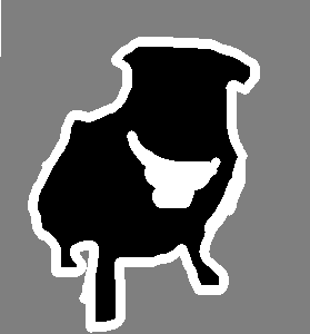
- View the results
Finally, let us visualize the results obtained.
# Generate predictions for all images in the validation set

val_gen = OxfordPets(batch_size, img_size, val_input_img_paths, val_target_img_paths)
val_preds = model.predict(val_gen)


def display_mask(i):
    """Quick utility to display a model's prediction."""
    mask = np.argmax(val_preds[i], axis=-1)
    mask = np.expand_dims(mask, axis=-1)
    img = PIL.ImageOps.autocontrast(keras.preprocessing.image.array_to_img(mask))
    display(img)


# Display results for validation image #10
i = 10

# Display input image
display(Image(filename=val_input_img_paths[i]))

# Display ground-truth target mask
img = PIL.ImageOps.autocontrast(load_img(val_target_img_paths[i]))
display(img)

# Display mask predicted by our model
display_mask(i)  # Note that the model only sees inputs at 150x150.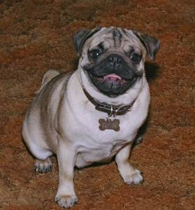
Conclusion:
The U-Net architecture is one of the most significant and revolutionary landmarks in the field of deep learning. While the initial research paper that introduced the U-Net architecture was to solve the task of Biomedical Image Segmentation, it was not limited to this single application. The model could and can still solve the most complex problems in deep learning. Although some of the elements in the original architecture are outdated, there are several variations of this architecture. These include LadderNet, U-Net with attention, the recurrent and residual convolutional U-Net (R2-UNet), and other similar networks which are derived successfully from the original U-Net Models.
In this article, we looked into a brief introduction of the U-Net modeling technique that finds fabulous utility in most modern tasks related to image segmentation. We then proceed to understand the construction and the main methodologies employed in the building of the U-Net architecture. We understood the numerous methodologies and techniques used to achieve the best results possible on the provided dataset. After this section, we learned how to build the U-Net architecture from scratch with various blocks to simplify the overall structure. Finally, we analyzed our constructed U-Net architecture with a simple example problem for image segmentation.
In the upcoming article, we will look into the CANet architecture for image segmentation and understand some of its core concepts. We will then proceed to build the entire architecture from scratch. Until then, have fun learning and exploring the world of Deep Learning!