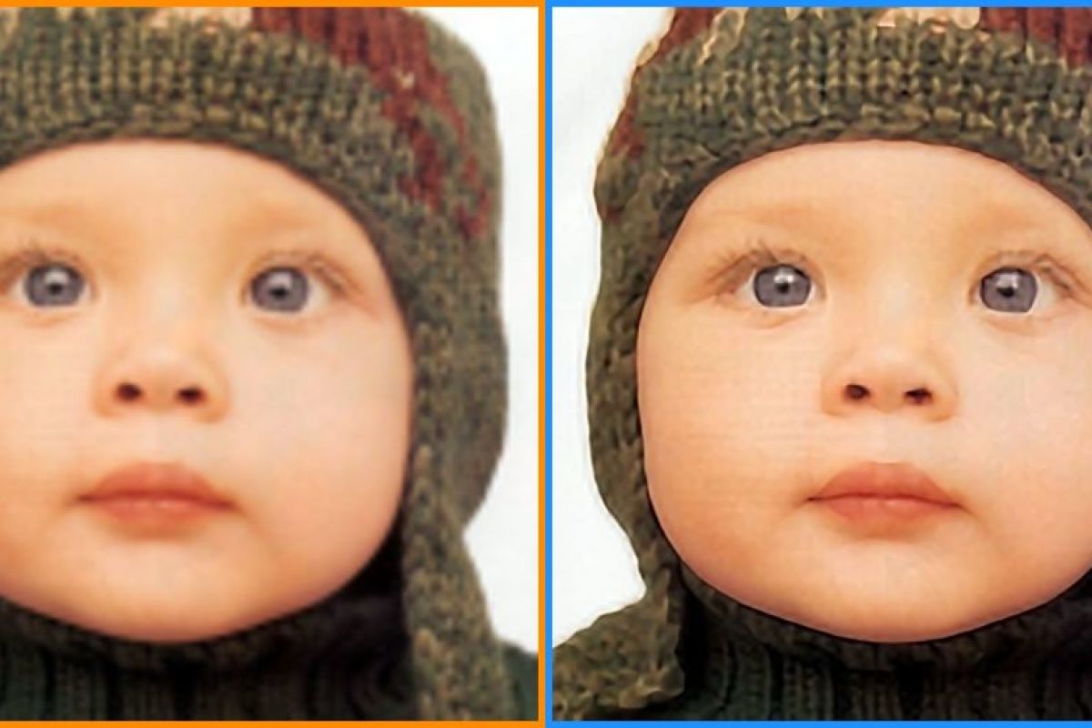
Image Super Resolution refers to the task of enhancing the resolution of an image from low-resolution (LR) to high (HR). It is popularly used in the following applications:

1. Surveillance: to detect, identify, and perform facial recognition on low-resolution images obtained from security cameras.
2. Medical: capturing high-resolution MRI images can be tricky when it comes to scan time, spatial coverage, and signal-to-noise ratio (SNR). Super resolution helps resolve this by generating high-resolution MRI from otherwise low-resolution MRI images.
3. Media: super resolution can be used to reduce server costs, as media can be sent at a lower resolution and upscaled on the fly.

Deep learning techniques have been fairly successful in solving the problem of image and video super-resolution. In this article we will discuss the theory involved, various techniques used, loss functions, metrics, and relevant datasets. You can also run the code for one of the models we'll cover, ESPCN, for free on the ML Showcase.

Image Super-Resolution

Low resolution images can be modeled from high resolution images using the below formula, where D is the degradation function, I_y is the high resolution image, I_x is the low resolution image, and $\sigma$ is the noise.

$$ I_{x} =  D(I_y; \sigma) $$

The degradation parameters D and $\sigma$ are unknown; only the high resolution image and the corresponding low resolution image are provided. The task of the neural network is to find the inverse function of degradation using just the HR and LR image data.

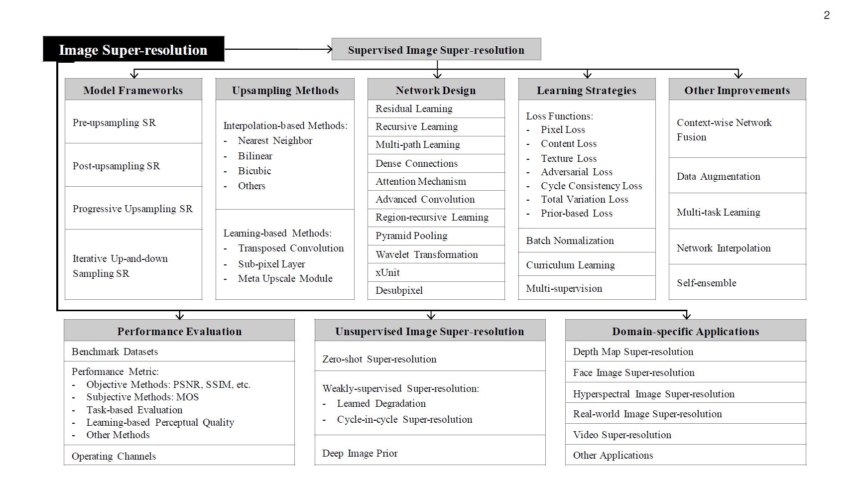
Super-Resolution Methods and Techniques

There are many methods used to solve this task. We will cover the following:

• Pre-Upsampling Super Resolution
• Post-Upsampling Super Resolution
• Residual Networks
• Multi-Stage Residual Networks
• Recursive Networks
• Progressive Reconstruction Networks
• Multi-Branch Networks
• Attention-Based Networks
• Generative Models

We'll look at several example algorithms for each.

Pre-Upsampling Super Resolution

The methods under this bracket use traditional techniques–like bicubic interpolation and deep learning–to refine an upsampled image.

The most popular method, SRCNN, was also the first to use deep learning, and has achieved impressive results.

SRCNN

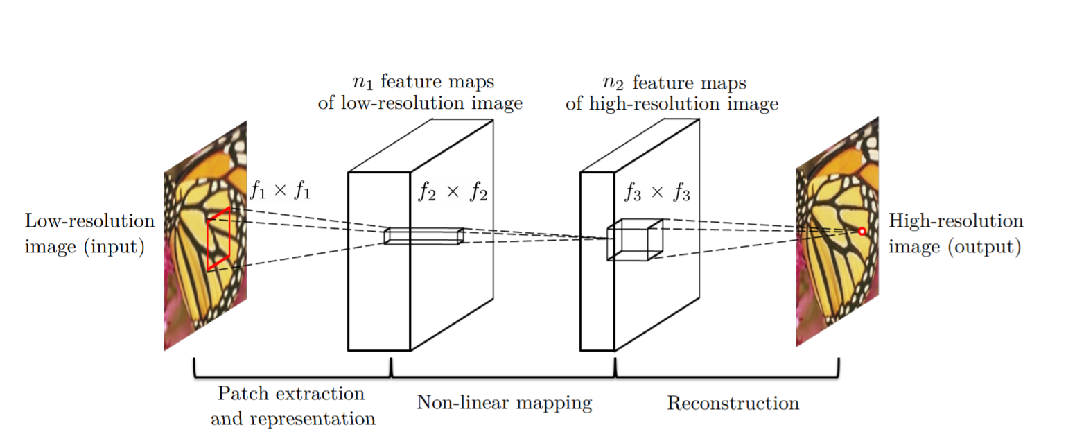
SRCNN is a simple CNN architecture consisting of three layers: one for patch extraction, non-linear mapping,​ and reconstruction. The patch extraction layer is used to extract dense patches from the input, and to represent​ them using convolutional filters. The non-linear mapping layer consists of 1×1 convolutional filters used to change the ​number of channels and add non-linearity. As you might have guessed, the final reconstruction layer reconstructs the high resolution image.

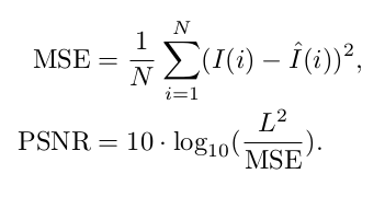
The MSE loss function is used to train the network, and PSNR (discussed below in the Metrics section) is used to evaluate the results. We ​will talk about both of these in more detail later on.

VDSR​

Very Deep Super Resolution (VDSR) is an improvement on SRCNN, with the addition of the following​ features:

• As the name signifies, a deep network with small 3×3 convolutional filters ​is used instead of a smaller network with large convolutional filters. This is based on the VGG architecture.
• The network tries to learn the residual of the output image and the interpolated input, rather​ than learning the direct mapping (like SRCNN), as shown in the figure above. This simplifies the task. The initial low resolution image is added to the network output to get the final HR output.
• Gradient clipping is used to train the deep network with higher learning rates.

Post-Upsampling Super-Resolution

Since the feature extraction process in pre-upsampling SR occurs in the high resolution space, the computational power required is also on the higher end. Post-upsampling SR tries to solve this by doing feature extraction in the lower resolution space, then doing upsampling only at the end, therefore significantly reducing computation. Also, instead of using simple bicubic interpolation for upsampling, a learned upsampling in the form of deconvolution/sub-pixel convolution is used, thus making the network trainable end-to-end.

Let's discuss a few popular techniques following this structure.

FSRCNN

As can be seen in the above figure, the major changes between SRCNN and FSRCNN are:

1. There is no pre-processing or upsampling at the beginning. The feature extraction took place in the low resolution space​.
2. A 1×1 convolution is used after the initial 5×5 convolution to reduce the number of channels, and hence ​lesser computation and memory, similar to how the Inception network is developed​.
3. Multiple 3×3 convolutions are used, instead of having a big convolutional filter, similar to how the VGG network works by simplifying the architecture to reduce the number of parameters.​
4. Upsampling is done by using a learned deconvolutional filter, thus improving the model.

FSRCNN ultimately achieves better results than SRCNN, while also being faster.

ESPCN

ESPCN introduces the concept of sub-pixel convolution to replace the deconvolutional layer for ​upsampling. This solves two problems associated with it:

1. Deconvolution happens in the high resolution space, and thus is more computationally expensive.
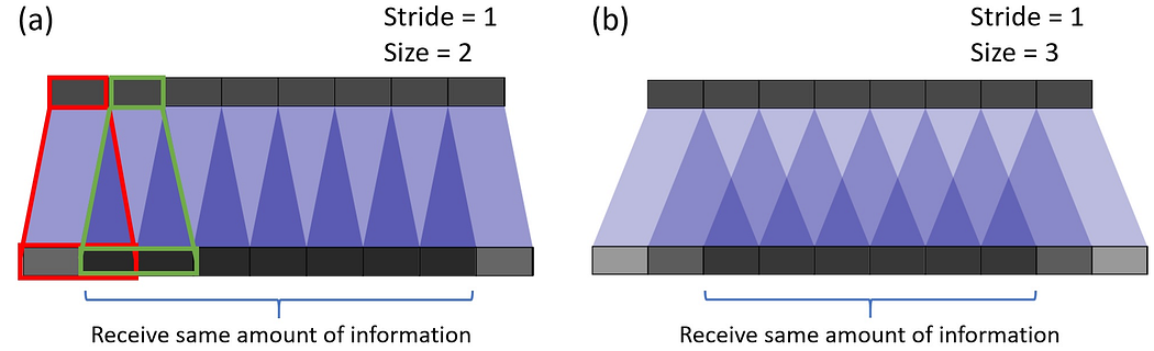
2. It resolves the checkerboard issue in deconvolution, which occurs due to the overlap​ operation of convolution (shown below)​.

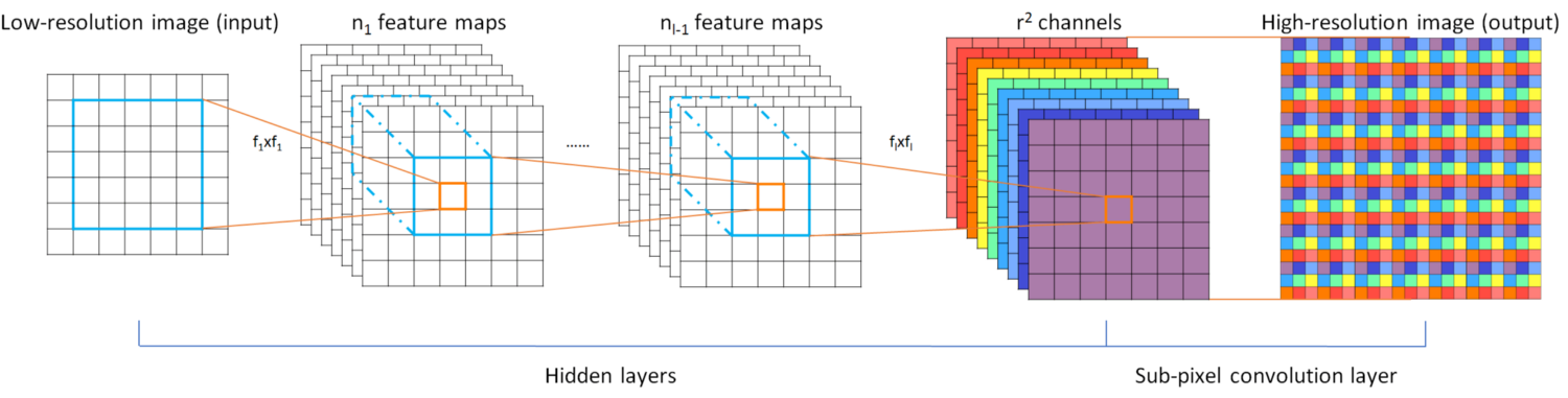
Sub-pixel convolution works by converting depth to space, as seen in the figure below. Pixels from multiple channels in a low resolution image are rearranged to a single channel in a high resolution image. To give an example, an input image of size 5×5×4 can rearrange the pixels in the final four channels to a single channel, resulting in a 10×10 HR image.

Let's now discuss a few more architectures which are based on the techniques from the figure below.

Residual Networks

EDSR

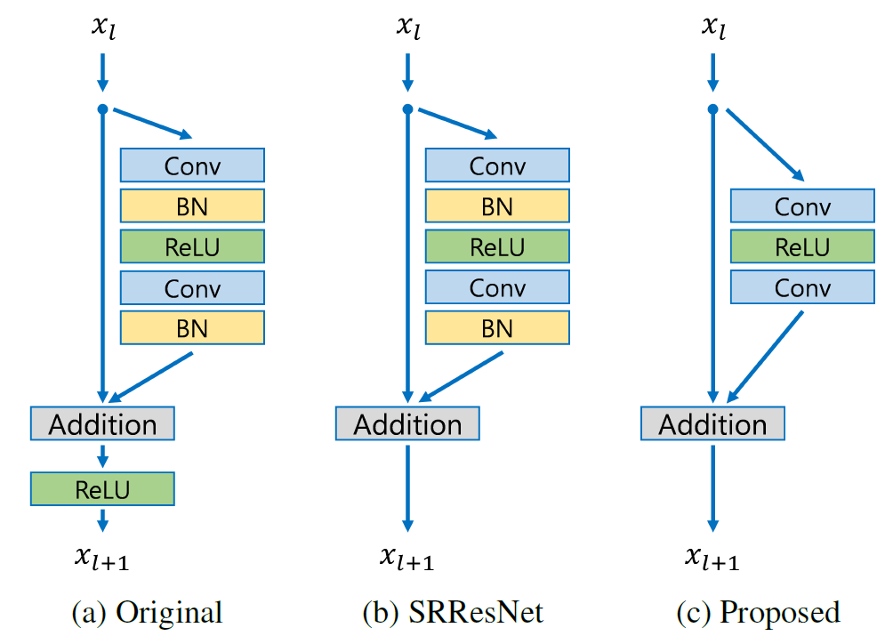
The EDSR architecture is based on the SRResNet architecture, consisting of multiple residual blocks. The residual block in EDSR is shown above. The major difference from SRResNet is that the Batch Normalization layers are removed. The author states that BN normalizes the input, thus limiting the range of the network; removal of BN results in an improvement in accuracy. The BN layers also consume memory, and removing them leads to up to a 40% memory reduction, making the network training more efficient.

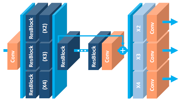
MDSR

MDSR is an extension of EDSR, with multiple input and output modules that give corresponding resolution outputs at 2x, 3x, and 4x. At the beginning, the pre-processing modules for scale-specific input are present consisting of two residual blocks with 5×5 kernels. A large kernel is used for the pre-processing layers to keep the network shallow, while still achieving a high receptive field. At the end of the scale-specific pre-processing modules are the shared residual blocks, which is a common block for data of all resolutions. Finally, after the shared residual blocks are the scale-specific upsampling modules. Although the overall depth of MDSR is 5x compared to single-scale EDSR, the number of parameters are only 2.5x, and not 5x, due to the shared parameters. MDSR achieves comparable results to scale-specific EDSR, even though the network has fewer parameters than the scale-specific EDSR models combined.

CARN

In the paper Fast, Accurate, and Lightweight Super-Resolution with Cascading Residual Network, the authors have proposed the following advancements on top of a traditional residual network:

1. A cascading mechanism at both the local and global level, to incorporate features from multiple layers and give the network the ability to receive more information.
2. In addition to CARN, a smaller CARN-M is proposed to have a lighter architecture, without much deterioration in results, with the help of recursive network architecture.

The global connections in CARN are visualized above. The culmination of each cascading block with a 1×1 convolution receives inputs from all the previous cascading blocks and the initial input, thus resulting in an effective transfer of information.

Every residual block in a cascading block ends in a 1x1 convolution which has connections from all previous residual blocks along with the main input, similar to how global cascading works.

The residual block in ResNet is replaced by a newly designed Residual-E block which is inspired from depthwise convolutions in MobileNet. Instead of depthwise convolutions, group convolutions are used, and the results show a decrease in 1.8-14x the number of computations used, depending on the group size.

To further reduce the number of parameters, a shared residual block is used (recursive block), thus resulting in less number of parameters by up to three times the original number. As can be seen in (d) above, a recursive shared block helps in reducing the total number of parameters.

Multi-Stage Residual Networks

To deal with the task of feature extraction separately in the low-resolution space and high-resolution space, a multi-stage design is considered in a few architectures to improve their performance. The first stage predicts the coarse features, while the later stage improves on it. Let's discuss an architecture involving one of these multi-stage networks.

BTSRN

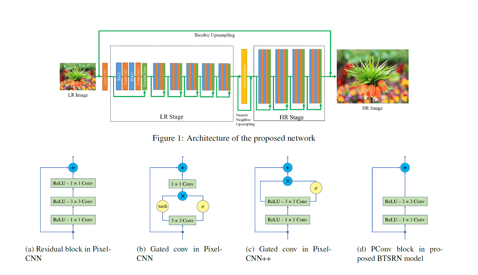
As can be seen in the above figure, BTSRN consists of two stages: a low resolution (LR) stage and a high resolution (HR) stage. The LR stage consists of 6 residual blocks, whereas the HR stage contains 4 residual blocks. Convolution in the HR stage requires more computation than in the LR stage, as the input size is higher. The number of blocks in both the stages are determined in such a way as to achieve a trade-off between accuracy and performance.

The output of the LR stage is upsampled before being sent to the HR stage. This is done by adding the outputs of the Deconvolution layer and Nearest Neighbor uspsampling.

The authors propose a novel residual block named PConv, as seen in (d) in the figure above. The proposed block achieves a good trade-off between accuracy and performance, based on the results.

Similar to EDSR, Batch Normalization is avoided to prevent re-centering and re-scaling, since it is found to be detrimental. This is due to the fact that super-resolution is a regression task, and thus target outputs are highly correlated with inputs' first-order statistics.

Recursive Networks

Recursive networks employ shared network parameters in convolutional layers to reduce their memory footprint, as seen in CARN-M above. Let's discuss a few more architectures involving recursive units.

DRCN

Deep Recursive Convolutional Network (DRCN) involves applying the same convolution layer multiple times. As can be seen in the figure above, the convolutional layers in the residual block are shared.

The outputs from all the intermediate shared convolutional blocks, along with the input, are sent to the reconstruction layer which generates the high resolution image using all of the inputs. Since there are multiple inputs used to generate the output, this architecture can be thought of as an ensemble of networks.

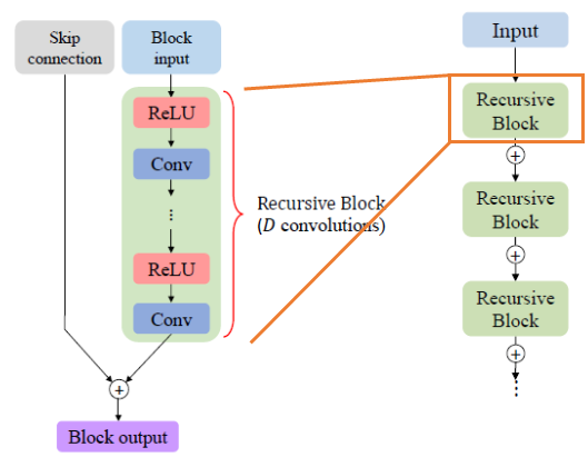
DRRN

Deep Recursive Residual Network (DRRN) is an improvement over DRCN by having residual blocks in the network over simple convolutional layers. The parameters in every residual block are shared with other residual blocks, as can be seen in the image above.

As you can see in the graph, DRRN outperforms SRCNN, ESPCN, VDSR, and DRCN, while having a comparable number of parameters.

Progressive Reconstruction Networks

CNNs in general give outputs in a single shot, but getting a high resolution image with a big scale factor (say 8x) is a tough task for a neural network. To solve this, some network architectures increase the resolution of images in steps. Now let's discuss a few networks which follow this style.

LAPSRN

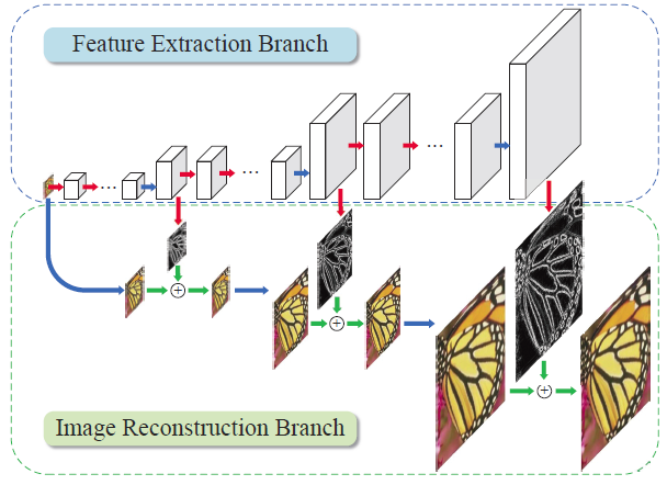
LAPSRN, or MS-LAPSRN, consists of a Laplacian pyramid structure which can upscale images to 2x, 4x, and 8x using a step-by-step approach.

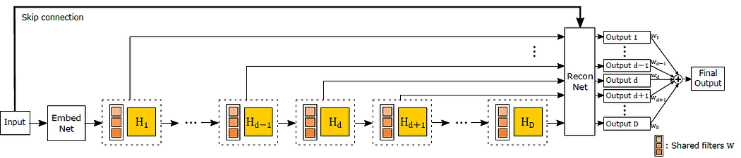
As can be seen in the above figure, LAPSRN consists of multiple stages. The network consists of two branches: the Feature Extraction Branch and the Image Reconstruction Branch. Each iterative stage consists of a Feature Embedding Block and Feature Upsampling Block, as seen in the figure below. The input image is passed through a feature embedding layer to extract features in the low resolution space, which is then upsampled using transpose convolution. The output learned is a residual image which is added to the interpolated input to get the high resolution image. The output of the Feature Upsampling Block is also passed to the next stage, which is used for refining the high resolution output of this stage and scaling it to the next level. Since lower-resolution outputs are used in refining further stages, there is shared learning which helps the network to perform better.

To reduce the memory footprint of the network, the parameters in Feature Embedding, Feature Upsampling, etc. are shared across the stages recursively.

Within the feature embedding block, individual residual block consists of shared convolution parameters (shown in the figure above) to further reduce the number of parameters.

The authors argued that since each LR input can have multiple HR representations, an L2 loss function produces a smoothed output over all representations, thus making the images not look sharp. To deal with this the Charbonnier loss function is used, which can handle outliers better.

Multi-branch networks

By now we've seen a trend: deeper networks give better results. But training deeper networks is tough due to the problem of information flow. Residual networks address this to an extent by using shortcut connections. Multi-branch networks work on improving information flow by having multiple branches through which information can pass, thus resulting in amalgamation of information from multiple receptive fields and hence better training. Let's discuss a few networks which employ this technique.

CMSC

Like other super-resolution frameworks, the Cascaded Multi-Scale Cross-Network (CMSC) has a feature extraction layer, cascaded sub-nets, and a reconstruction layer–shown below.

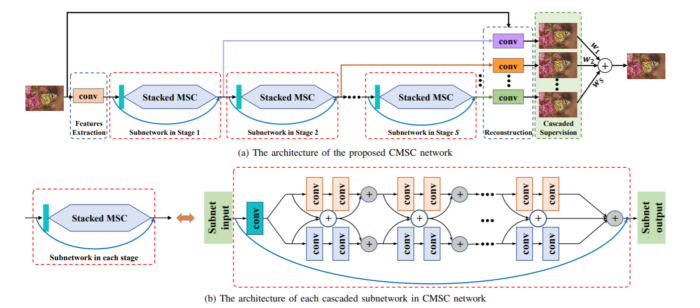
The cascaded sub-network consists of two branches, as can be seen in (b). Each branch has different sizes of filters, and hence results in a different receptive field. Fusion of information from different receptive fields across the module results in better information flow. Multiple blocks of MSC's are stacked one after another to gradually decrease the difference between the output and HR image iteratively. The outputs from all the blocks are passed together to a reconstruction block to get the final HR output.

IDN

Information Distillation Network (IDN) is proposed to achieve fast and accurate results for the task of super-resolution. Like other multi-branch networks, IDN utilizes the capability of multiple branches to improve the information flow in a deep network.

The IDN architecture consists of FBlock to do feature extraction, multiple DBlocks, and RBlock to do transposed convolution to achieve learned upscaling. The contribution of the paper is in the DBlock, which consists of two units: the Enhancement Unit and Compression Unit.

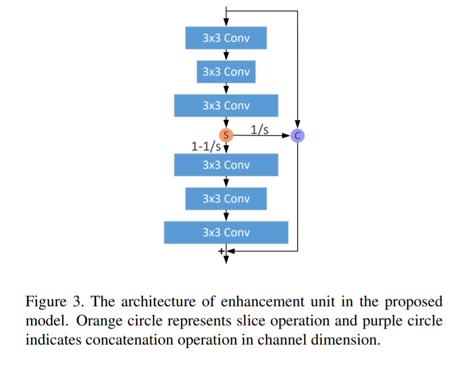
Enhancement unit's structure is shown in the figure above. Input is passed through three convolutional filters of size 3×3, and is then sliced. One part of the slice is concatenated with the initial input to pass via shortcut connection to the final layer. The remaining slice is passed through another set of convolutional filters of size 3×3. The final output is generated by summing up both the inputs and final layer. Having this kind of structure helps in capturing both the short-range information and the long-range information at the same time.

The compression unit takes the output of the enhancement unit and passes it through a 1×1 convolutional filter to compress (or reduce) the number of channels.

Attention-Based Networks

The networks discussed so far give equal importance to all spatial locations and channels. In general, giving selective attention to different regions in an image can give much better results. We shall now discuss few architectures which help in achieving this.

SelNet

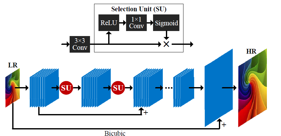
SelNet proposes a novel Selection unit at the end of convolutional blocks which help to decide which information to pass on, selectively. A Selection Module consists of a ReLu activation followed by 1×1 convolution and sigmoid gating. A Selection Unit is the multiplication of a Selection Module and an identity connection.

A sub-pixel layer (similar to ESPCN) is kept towards the end of the network to achieve learned upscaling. The network learns a residual HR image, which is then added to the interpolated input to get the final HR image.

RCAN

All through this article we have observed that having deeper networks improves performance. In order to train deeper networks, Residual Channel Attention Networks (RCAN) suggest RIR modules with Channel attention. Let's discuss these more in detail.

The input in RCAN is passed through a single convolutional filter for feature extraction, which is then bypassed towards the final layer with a long skip connection. The long skip connection is added to carry the low frequency signals from the LR image while the main network (i.e RIR) focuses on capturing the high frequency information.

RIR consists of multiple RG blocks, each having a structure shown in the above figure. Each RG block has multiple RCAB modules along with a skip connection, referred to as a short skip connection, to help transfer the low frequency signal.

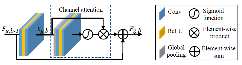
RCAB has a structure (as shown above) comprised of a GAP module to achieve channel attention, similar to the Squeeze and Excite blocks in SqueezeNet. The channel-wise attention is multiplied with the output from the sigmoid gating function of a convolutional block. This output is then added to the shortcut input connection to get the final output value of a RCAB block.

Generative Models

The networks discussed so far optimize the pixel difference between predicted and output HR images. Although this metric works fine, it is not ideal; humans don't distinguish images by pixel difference, but rather by perceptual quality. Generative models (or GANs) try to optimize the perceptual quality to produce images which are pleasant to the human eye. Finally, let's take a look at a few GAN-related architectures.

SRGAN

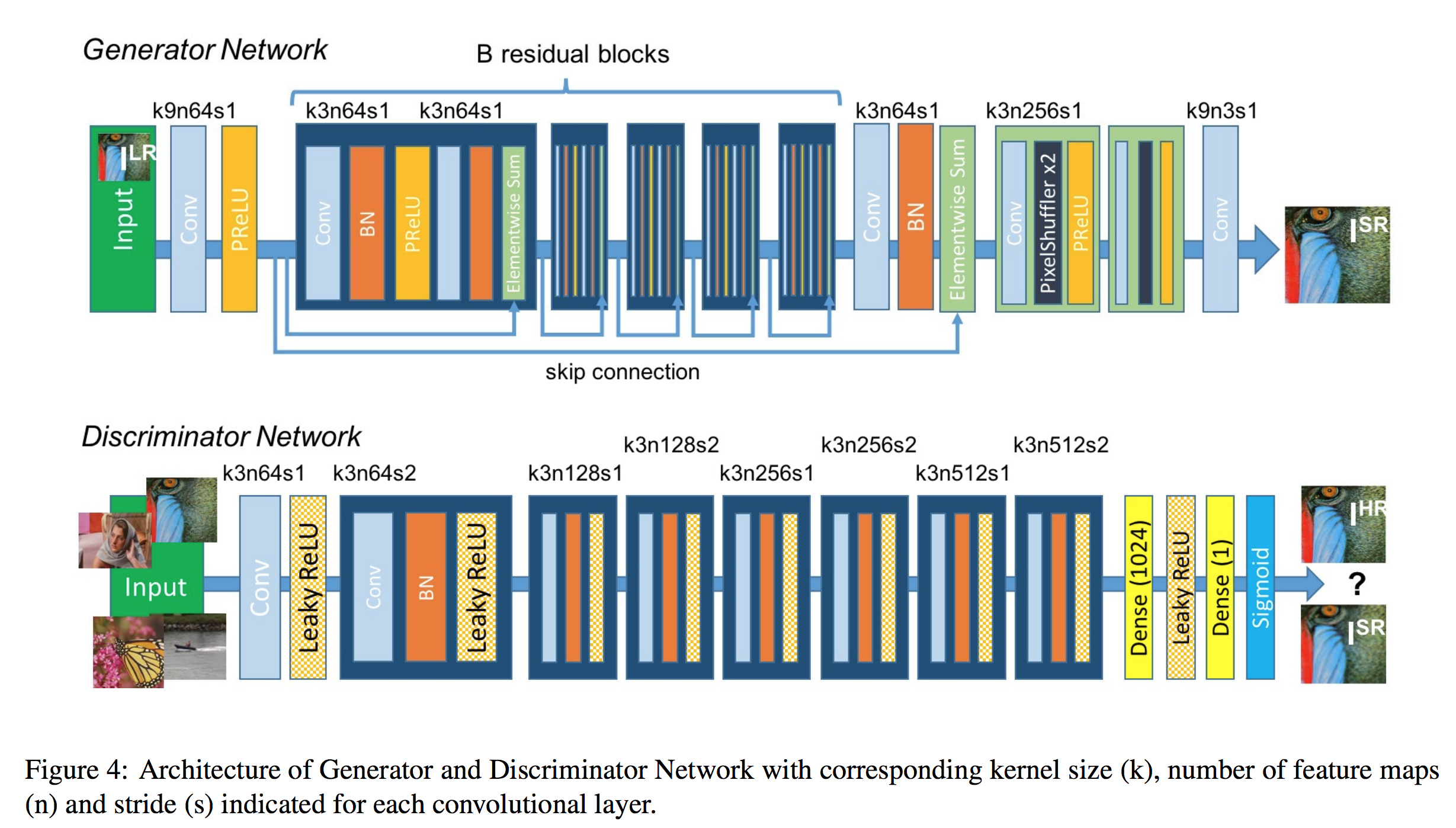
SRGAN uses a GAN-based architecture to generate visually pleasing images. It uses the SRResnet network architecture as a backend, and employs a multi-task loss to refine the results. The loss consists of three terms:

1. MSE loss capturing pixel similarity
2. Perceptual similarity loss, which is used to capture high-level information by using a deep network
3. Adversarial loss from the discriminator

Although the results obtained had comparatively lower PSNR values, the model achieved more MOS, i.e a better perceptual quality in the results.

EnhanceNet

EnhanceNet uses a Fully Convolutional Network with residual learning, which employs an extra term in the loss function to capture finer texture information. In addition to the above described losses in SRGAN, a texture loss similar to the one in Style Transfer is employed to capture the finer texture information.

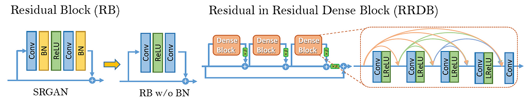
ESRGAN

ESRGAN improves on top of SRGAN by adding a relativistic discriminator. The advantage is that the network is trained not only to tell which image is true or fake, but also to make real images look less real compared to the generated images, thus helping to fool the discriminator. Batch normalization in SRGAN is also removed, and Dense Blocks (inspired from DenseNet) are used for better information flow. These Dense Blocks are called RRDB.

Datasets

The following are some of the common datasets used to train super-resolution networks.

1. DIV2K:  800 train, 100 validation, and 100 test. 2K resolution images are provided, including both high and low resolution images with 2x, 3x, and 4x downscaling factors. Proposed in the NTIRE17 challenge.
2. Flickr2K: 2650 2K images from FLICKR.
3. Waterloo: The Waterloo Exploration Database contains 4,744 pristine natural images and 94,880 distorted images created from them.

Loss Functions

In this section we shall discuss various loss functions which can be used to train the networks.

1. Pixel Loss: This is the most simple and common type of loss function used in training super-resolution networks. L2, L1, or some difference metric is used to evaluate the model. Training with pixel loss optimizes PSNR, but doesn't directly optimize the perceptual quality, and hence generates images which might not be pleasing to the human eye.
2. Perceptual Loss: Perceptual loss tries to match the high-level features in a generated image with a given HR output image. This is achieved by taking a pre-trained network, like VGG, and using the difference of feature outputs between predicted and output images as loss. This loss function is introduced in SRGAN.
3. Charbonnier Loss: This loss function is used in LapSRN instead of the generic L2 loss. The results show that Charbonnier loss deals better with outliers and produces sharper images compared to those generated with L2 loss, which are generally smoother.
4. Texture Loss: Introduced in EnhanceNet, this loss function tries to optimize the Gram matrix of feature outputs inspired by the Style Transfer loss function. This loss function trains the network to capture the texture information in a HR image.
5. Adversarial Loss: Used in all GAN-related architectures, adversarial loss helps in fooling the discriminator and generally produces images which have better perceptual quality. ESRGAN adds an extra variant of this by using the relativistic discriminator, and thus instructing the network not only to make fake images more real, but also to make real images look more fake.

Metrics

In this section we shall discuss the various metrics used to compare the performance of various models.

1. PSNR: Peak Signal to Noise Ratio is the most common technique used to determine the quality of results. It can be calculated directly from the MSE using the formula below, where L is the maximum pixel value possible (255 for an 8-bit image).

2.  SSIM: This metric is used to compare the perceptual quality of two images using the formula below, with the mean ($\mu$), variance ($\sigma$), and correlation (c) of both images.

3. MOS: Mean Opinion Score is a manual way to determine the results of a model, where humans are asked to rate an image between 0 and 5. The results are aggregated and the average result is used as a metric.

By this point you might be like:

Let's code one of the popular architectures we have discussed so far, ESPCN.

inputs = keras.Input(shape=(None, None, 1))
conv1 = layers.Conv2D(64, 5, activation="tanh", padding="same")(inputs)
conv2 = layers.Conv2D(32, 3, activation="tanh", padding="same")(conv1)
conv3 = layers.Conv2D((upscale_factor*upscale_factor), 3, activation="sigmoid", padding="same")(conv2)
outputs = tf.nn.depth_to_space(conv3, upscale_factor, data_format='NHWC')
model = Model(inputs=inputs, outputs=outputs)

As we know, ESPCN consists of convolutional layers for feature extraction followed by sub-pixel convolution for upsampling. We are using the TensorFlow depth_to_space function to perform sub-pixel convolution.

def gen_dataset(filenames, scale):
    # The model trains on 17x17 patches
    crop_size_lr = 17
    crop_size_hr = 17 * scale

    for p in filenames:
        image_decoded = cv2.imread("Training/DIV2K_train_HR/"+p.decode(), 3).astype(np.float32) / 255.0
        imgYCC = cv2.cvtColor(image_decoded, cv2.COLOR_BGR2YCrCb)
        cropped = imgYCC[0:(imgYCC.shape[0] - (imgYCC.shape[0] % scale)),
                  0:(imgYCC.shape[1] - (imgYCC.shape[1] % scale)), :]
        lr = cv2.resize(cropped, (int(cropped.shape[1] / scale), int(cropped.shape[0] / scale)),
                        interpolation=cv2.INTER_CUBIC)

        hr_y = imgYCC[:, :, 0]
        lr_y = lr[:, :, 0]

        numx = int(lr.shape[0] / crop_size_lr)
        numy = int(lr.shape[1] / crop_size_lr)
        for i in range(0, numx):
            startx = i * crop_size_lr
            endx = (i * crop_size_lr) + crop_size_lr
            startx_hr = i * crop_size_hr
            endx_hr = (i * crop_size_hr) + crop_size_hr
            for j in range(0, numy):
                starty = j * crop_size_lr
                endy = (j * crop_size_lr) + crop_size_lr
                starty_hr = j * crop_size_hr
                endy_hr = (j * crop_size_hr) + crop_size_hr

                crop_lr = lr_y[startx:endx, starty:endy]
                crop_hr = hr_y[startx_hr:endx_hr, starty_hr:endy_hr]

                hr = crop_hr.reshape((crop_size_hr, crop_size_hr, 1))
                lr = crop_lr.reshape((crop_size_lr, crop_size_lr, 1))
                yield lr, hr

We will be using the DIV2K dataset to train the model. We split the 2k resolution images into patches of 17×17 to provide as model input for training. The authors convert RGB images to the YCrCb format, and then upscale the Y channel input using ESPCN. The Cr and Cb channels are upscaled using bicubic interpolation, and all the upscaled channels are stitched together to get the final HR image. Thus, while training, we only need to provide the Y channel of the low resolution data and the high resolution images to the model.

The full code can be run for free on Gradient in a Gradient Community (Jupyter) Notebook.

Summary

In this article we covered what super-resolution is, its applications, the taxonomy of super-resolution algorithms, along with their advantages and limitations. Then we took a look at some of the publicly available datasets to get started with, as well as the different kinds of loss functions and metrics which can be used. Finally we went though the code for the ESPCN architecture.

If you want to keep learning about super-resolution, I recommend this repo which includes a collection of research papers and links to their corresponding code.