The optimization of deep learning algorithms and frameworks is a question not only of libraries and techniques, but also of CPU and GPU hardware. How data is stored in terms of computer number format, for example, can have significant effects on the training speed of a deep learning algorithm. This information is especially useful to know when using GPUs to accelerate model training.
In this blogpost, we'll introduce two common computer number formats used for deep learning (FP16 and FP32) and detail the issues with using each alone. Next, we'll jump into the benefits of mixed precision training and its use in deep learning. After that, we'll break down which NVIDIA GPUs are capable of automatic mixed precision training including what kinds of speedups you might expect when implementing mixed precision training on various GPUs, how to make sure mixed precision is enabled whether you're running PyTorch or TensorFlow, and then why mixed precision is especially valuable if you're running on powerful GPUs like the NVIDIA RTX5000, V100, or A100.
What are computer number formats, and how do they affect deep learning?
Computer number formats are internal representations of numeric values in digital device hardware and software. These representations can be operated on by code and applications to be used in tasks.
As set out in the international standard for computer number formats, IEEE 754, there are various levels of floating-point precision. These range from FP16 to FP256, where the number after the "FP" (Floating Point) represents the number of bits available for representing the floating-point value. (1)
In deep learning tasks, float32, also known as FP32, is historically the most popular computer number format to use with deep learning tasks. This is because in FP32, a single bit is reserved for the sign, 8 bits are reserved for the exponent (-126 to +127), and 23 bits for the digits. FP16, which represents half precision, reserves one bit for the sign, 5 more bits for the exponent (-14 to +14), and 10 for the digits. (1)

The consequence of using either of these two formats for deep learning can be seen in their minimum and maximum representation values and the corresponding effect these sizes have on memory. The differences between the minimum and maximum of each format are on the order of > 10^30 in magnitude of difference. This means that a far wider range of values can be represented in FP32 than FP16, althought that comes at the cost of significantly more bits for each single value stored.
The consequences of these differences in representative capability are shown in two places: speed and efficacy. In effect, using FP32 will lead to a better overall model due to the higher numerical precision of the numbers used in the deep learning operation, but it will also take significantly more memory. Despite the higher cost, the higher accuracy has made FP32 the lingua franca for storing numerical values for deep learning tasks.
On the other hand, deep learning with FP16 takes less memory and runs more quickly, but with less precision in the data and a resultant loss in model efficacy. Furthermore, modern accelerator hardware like Google TPUs and NVIDIA GPUs run operations faster in the 16-bit dtypes. This is because they have specialized hardware to run 16-bit computations and 16-bit dtypes can be read from memory more quickly than FP32. Despite the speedup benefits, the loss in data precision and model accuracy is often too much to make FP16 viable in all but niche situations.
What is mixed precision training?
In the past, the most commonly used precision training paradigm was single precision training with FP32. This is because the overall efficacy of the model is consistently higher with FP32 although it comes at the cost of increased memory and training time requirements. Mixed precision training emerged as a way to try to capture the efficacy of FP32 with the efficiency of FP16.
In general, mixed precision training provides three key benefits to deep learning:
- Using Tensor Cores to process FP16 speeds up math-intensive operations like those in linear or convolution layers
- Accessing half the bytes compared to single precision allows for increased speed on memory-limited operations
- Lowering the memory requirements to train models, and thus enable the training of larger models or the use of larger minibatches (2)
Let's look at how mixed precision training can create these benefits by looking at the theory behind the paradigm.
Theory of mixed precision training in deep learning

In 2017, researchers at NVIDIA released a paper on mixed precision training. This paper detailed the first method for using both FP32 and FP16 for deep learning in a process called mixed precision training. As shown in the diagram above, they did this by first creating a a permanent copy of the weights stored in FP32. This is then converted into FP16 during the forward pass, to be used by the model to calculate the gradients, which are then converted to FP32, and passed back to the optimizer for back propagation. At the end of the iteration, the gradients in FP32 are used to update the master weights during the optimizer step.
The problem with the method alone is that there still remained some small gradients unaccounted for by FP16. The NVIDIA team found that there were values ranging between 2^-27 and 2^-24 which would affect training if made inviable. Because they were outside of the limit of FP16, they would be equated to zero during the training iteration. The solution to this was loss scaling – a process by which the loss value is multiplied by a scaling factor after the forward pass is completed and before back-propagation. Using the chain rule, all the gradients are subsequently scaled by the same factor and subsequently moved within the range of viability for FP16. (1)
Mixed precision training in practice
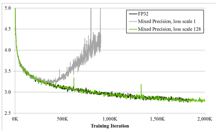
The effect of using mixed precision training can be seen in the plotting diagram above. It details the training curves for the big LSTM English language model when using the three different precision formats: FP32, Mixed precision with a loss scale of 1, and mixed precision with a loss scale of 128. The Y-axis is training loss, and we can use it to see how mixed precision without loss scaling (grey) diverges after a while, whereas mixed precision with loss scaling (green) matches the single precision model (black). (3) This shows clearly that mixed precision training with loss scaling can achieve nearly identical performance to single precision FP32.
Automatic mixed precision training
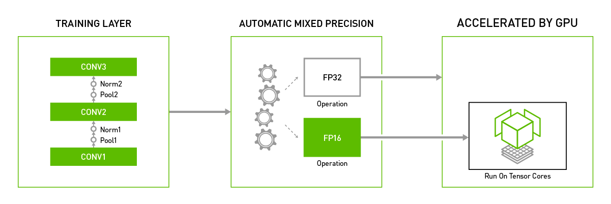
In the real world, much has changed since these topics were originally introduced. Most deep learning libraries now come equipped with the ability to use automatic mixed precision (AMP) training. Automatic mixed precision training is where mixed precision training is toggled on for a deep learning task without any additional set up by the user. Notably, PyTorch and TensorFlow both have built-in triggers for automatic mixed training.
Automatic mixed precision training in PyTorch
To enable PyTorch AMP, add the following lines to your code:
scaler = GradScaler()

with autocast():
    output = model(input)
    loss = loss_fn(output, target)

scaler.scale(loss).backward()

scaler.step(optimizer)

scaler.update()
Automatic mixed precision training in TensorFlow:
To use AMP with TensorFlow, simply wrap the tf.train or tf.keras.optimizers in the following to apply automatic loss scaling an automatic casting to half precision:
opt = tf.train.experimental.enable_mixed_precision_graph_rewrite(opt)For more information about Automatic Mixed Precision training, check out this official resource from NVIDIA.
When should you use mixed precision training on Gradient notebooks?
So far, we've discussed what mixed precision training is, shown the theory behind its mechanisms, and talked about how to use it automatically with the most popular deep learning libraries. Because mixed precision training is capable of accelerating general processes with deep learning tasks, we can already infer that it should be implemented wherever possible. But that's not always possible – especially in the context of automatic mixed precision training. In this section we will talk about where and when to make use of mixed precision training on Gradient Notebooks.
The problem of where and when automatic mixed precision training can be used on Gradient lies with hardware. Not all NVIDIA GPUs can be used with mixed precision training. GPUs with a compute capability of 7.0 and higher see the greatest performance benefit from using AMP. Newer GPUs have Tensor Cores which can accelerate FP16 matrix multiplications and convolutions, while older GPUs may still experience speedups related to memory and bandwidth. GPUs like the RTX5000, V100, and A100 will receive the most benefits from automatic mixed precision thanks to the Tensor Cores. If you are working with these machines, you should always enable automatic mixed precision training.
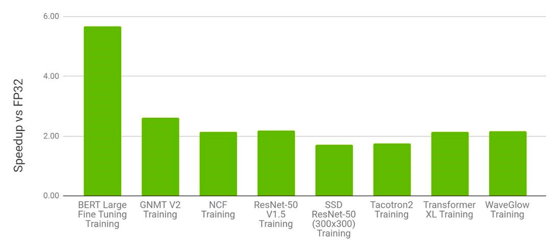
Above is a diagram from the official PyTorch blogpost about AMP with Torch. They found that particularly large models like BERT large could experience nearly a 6x improvement in training times when compared against single precision training methods while training on a 8 x V100 multi-GPU machine. We can also see that across the board, automatic mixed precision training can nearly halve training times compared to FP32 training.
In their next example, they detailed the comparative speedup factors between the V100 and A100. For some context, the A100 is widely considered a premiere machine for performing production grade deep learning tasks. The V100 is in many ways its predecessor in the deep learning community. The V100 is a powerful machine in its own right, but it is of an older design and make than the A100. As a result, by comparing the relative speedups between using automatic mixed precision training and single precision training with these two GPUs, we can see how much of an impact microarchitecture has on accelerating training when using AMP training.
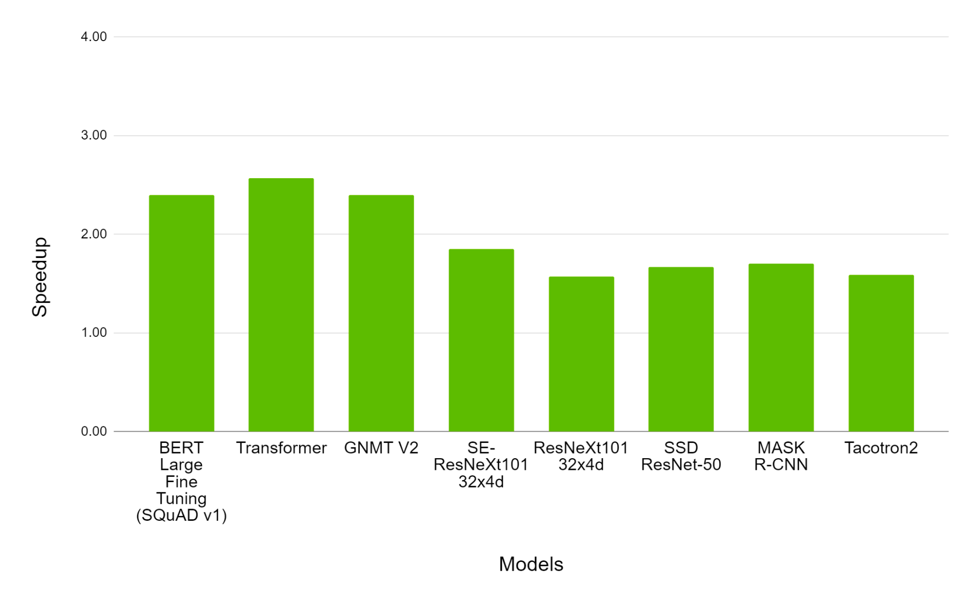
As we can see, the effect of the speedup for the A100 ranges from ~150% to ~250% speedup greater than the magnitude of the speedup in the V100. This shows, once again, not only the superiority of the A100 for deep learning tasks, but also how the advancements in microarchitecture and corresponding upgrades to the Tensor Core technology can affect training times.
Using automatic mixed precision training is something we should always be doing on any RTX, Tesla, and Ampere GPU, but the benefits will be most visible in the most powerful GPUs on the largest models.
Concluding thoughts
From the collected information above, we can see that mixed precision training should be implemented wherever possible. The advantages in terms of speedup are extremely high with very little drawback in terms of efficacy of the model. Furthermore, users of Gradient should be applying automatic mixed precision training whenever using an RTX, Tesla, or Ampere GPU. These GPUs have Tensor Cores which accelerate calculations being done with FP16.
For more information about computer number formats, mixed precision training, and AMP training with PyTorch and TensorFlow, read the links below:
- https://developer.nvidia.com/automatic-mixed-precision
- https://towardsdatascience.com/understanding-mixed-precision-training-4b246679c7c4
- https://developer.nvidia.com/blog/mixed-precision-training-deep-neural-networks/
- https://pytorch.org/blog/accelerating-training-on-nvidia-gpus-with-pytorch-automatic-mixed-precision/

